Lecture 7: Smoothing

Rafael A. Irizarry and Hector Corrada Bravo

March, 2010

Kernel Methods

Below is the results of using running mean (K nearest neighbor) to estimate theeffect of time to zero conversion on CD4 cell count.

Figure 1: Running mean estimate: CD4 cell count since zeroconversion for HIVinfected men.

One of the reasons why the running mean (seen in Figure 1) is wiggly is becausewhen we move from xi to xi+1 two points are usually changed in the group

1

we average. If the new two points are very different then s(xi) and s(xi+1)may be quite different. One way to try and fix this is by making the transitionsmoother. That’s one of the main goals of kernel smoothers.

Kernel Smoothers

Generally speaking a kernel smoother defines a set of weights Wi(x)ni=1 foreach x and defines

f(x) =n∑

i=1

Wi(x)yi. (1)

Most smoothers can be considered to be kernel smoothers in this very generaldefinition. However, what is called a kernel smoother in practice has a simpleapproach to represent the weight sequence Wi(x)ni=1: by describing the shapeof the weight function Wi(x) via a density function with a scale parameter thatadjusts the size and the form of the weights near x. It is common to refer tothis shape function as a kernel K. The kernel is a continuous, bounded, andsymmetric real function K which integrates to one:

∫K(u) du = 1.

For a given scale parameter h, the weight sequence is then defined by

Whi(x) =K(

x−xi

h

)∑ni=1K

(x−xi

h

)Notice:

∑ni=1Whi(xi) = 1

The kernel smoother is then defined for any x as before by

f(x) =n∑

i=1

Whi(x)Yi.

Because we think points that are close together are similar, a kernel smootherusually defines weights that decrease ina smooth fashion as one moves away from the target point.

Running mean smoothers are kernel smoothers that use a “box” kernel. A natu-ral candidate for K is the standard Gaussian density. (This is very inconvenientcomputationally because its never 0). This smooth is shown in Figure 2 forh = 1 year.

In Figure 3 we can see the weight sequence for the box and Gaussian kernelsfor three values of x.

2

Figure 2: CD4 cell count since zeroconversion for HIV infected men.

3

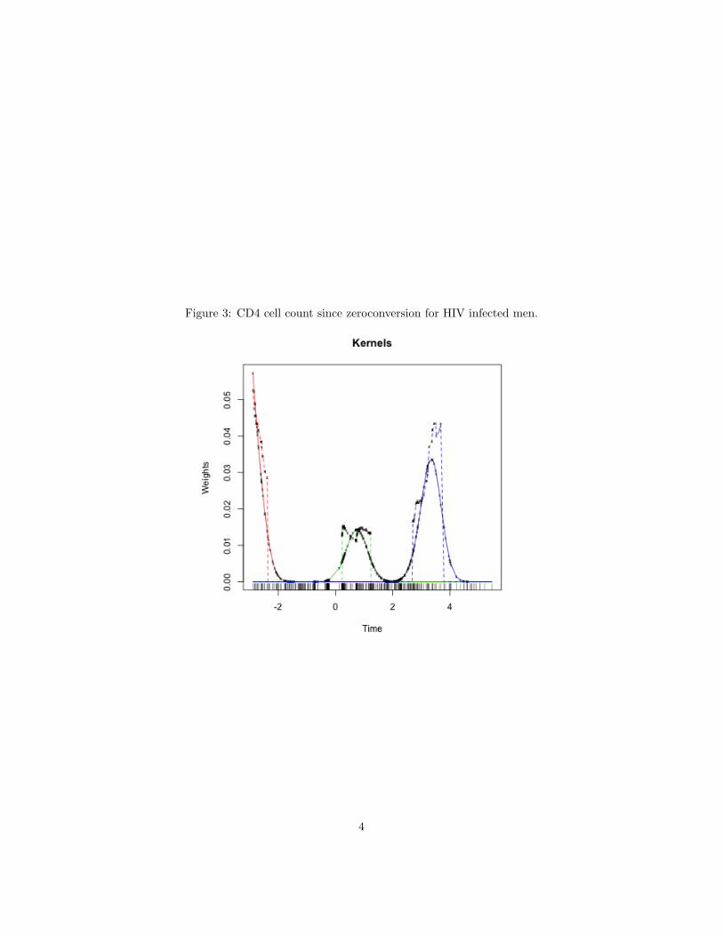
Figure 3: CD4 cell count since zeroconversion for HIV infected men.

4

Technical Note: An Asymptotic result

For the asymptotic theory presented here we will assume the stochastic designmodel with a one-dimensional covariate.

For the first time in this Chapter we will set down a specific stochastic model.Assume we have n IID observations of the random variables (X,Y ) and that

Yi = f(Xi) + εi, i = 1, . . . , n (2)

where X has marginal distribution fX(x) and the εi IID errors independent ofthe X. A common extra assumption is that the errors are normally distributed.We are now going to let n go to infinity. . . What does that mean?

For each n we define an estimate for f(x) using the kernel smoother with scaleparameter hn.

Theorem 1. Under the following assumptions

1.∫|K(u)| du <∞

2. lim|u|→∞ uK(u) = 0

3. E(Y 2) ≤ ∞

4. n→∞, hn → 0, nhn →∞

Then, at every point of continuity of f(x) and fX(x) we have∑ni=1K

(x−xi

h

)yi∑n

i=1K(

x−xi

h

) → f(x) in probability.

Proof : Optional homework. Hint: Start by proving the fixed design model.

Local Regression

Local regression is used to model a relation between a predictor variable andresponse variable. To keep things simple we will consider the fixed design model.We assume a model of the form

Yi = f(xi) + εi

where f(x) is an unknown function and εi is an error term, representing randomerrors in the observations or variability from sources not included in the xi.

We assume the errors εi are IID with mean 0 and finite variance var(εi) = σ2.

We make no global assumptions about the function f but assume that locally itcan be well approximated with a member of a simple class of parametric func-tion, e.g. a constant or straight line. Taylor’s theorem says that any continuousfunction can be approximated with polynomial.

5

Techinical note: Taylor’s theorem

We are going to show three forms of Taylor’s theorem.

• This is the original. Suppose f is a real function on [a, b], f (K−1) iscontinuous on [a, b], f (K)(t) is bounded for t ∈ (a, b) then for any distinctpoints x0 < x1 in [a, b] there exist a point x between x0 < x < x1 suchthat

f(x1) = f(x0) +K−1∑k=1

f (k)(x0)k!

(x1 − x0)k +f (K)(x)K!

(x1 − x0)K .

Notice: if we view f(x0) +∑K−1

k=1f(k)(x0)

k! (x1−x0)k as function of x1, it’sa polynomial in the family of polynomials

PK+1 = f(x) = a0 + a1x+ · · ·+ aKxK , (a0, . . . , aK)′ ∈ RK+1.

• Statistician sometimes use what is called Young’s form of Taylor’s Theo-rem:

Let f be such that f (K)(x0) is bounded for x0 then

f(x) = f(x0) +K∑

k=1

f (k)(x0)k!

(x− x0)k + o(|x− x0|K), as |x− x0| → 0.

Notice: again the first two term of the right hand side is in PK+1.

• In some of the asymptotic theory presented in this class we are going touse another refinement of Taylor’s theorem called Jackson’s Inequality:

Suppose f is a real function on [a, b] with K is continuous derivatives then

ming∈Pk

supx∈[a,b]

|g(x)− f(x)| ≤ C(b− a

2k

)K

with Pk the linear space of polynomials of degree k.

Fitting local polynomials

Local weighter regression, or loess, or lowess, is one of the most popular smooth-ing procedures. It is a type of kernel smoother. The default algorithm for loessadds an extra step to avoid the negative effect of influential outliers.

We will now define the recipe to obtain a loess smooth for a target covariate x0.

The first step in loess is to define a weight function (similar to the kernel K wedefined for kernel smoothers). For computational and theoretical purposes we

6

will define this weight function so that only values within a smoothing window[x0 + h(x0), x0 − h(x0)] will be considered in the estimate of f(x0).

Notice: In local regression h(x0) is called the span or bandwidth. It is likethe kernel smoother scale parameter h. As will be seen a bit later, in localregression, the span may depend on the target covariate x0.

This is easily achieved by considering weight functions that are 0 outside of[−1, 1]. For example Tukey’s tri-weight function

W (u) =

(1− |u|3)3 |u| ≤ 10 |u| > 1.

The weight sequence is then easily defined by

wi(x0) = W

(xi − x0

h(x)

)

We define a window by a procedure similar to the k nearest points. We wantto include α× 100% of the data.

Within the smoothing window, f(x) is approximated by a polynomial. Forexample, a quadratic approximation

f(x) ≈ β0 + β1(x− x0) +12β2(x− x0)2 for x ∈ [x0 − h(x0), x0 + h(x0)].

For continuous function, Taylor’s theorem tells us something about how goodan approximation this is.

To obtain the local regression estimate f(x0) we simply find the β = (β0, β1, β2)′

that minimizes

β = arg minβ∈R3

n∑i=1

wi(x0)[Yi − β0 + β1(xi − x0) +12β2(xi − x0)]2

and define f(x0) = β0.

Notice that the Kernel smoother is a special case of local regression. Provingthis is a Homework problem.

Defining the span

In practice, it is quite common to have the xi irregularly spaced. If we havea fixed span h then one may have local estimates based on many points andothers is very few. For this reason we may want to consider a nearest neighborstrategy to define a span for each target covariate x0.

7

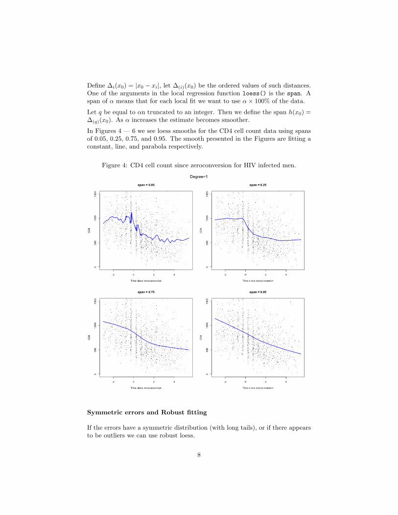
Define ∆i(x0) = |x0 − xi|, let ∆(i)(x0) be the ordered values of such distances.One of the arguments in the local regression function loess() is the span. Aspan of α means that for each local fit we want to use α× 100% of the data.

Let q be equal to αn truncated to an integer. Then we define the span h(x0) =∆(q)(x0). As α increases the estimate becomes smoother.

In Figures 4 — 6 we see loess smooths for the CD4 cell count data using spansof 0.05, 0.25, 0.75, and 0.95. The smooth presented in the Figures are fitting aconstant, line, and parabola respectively.

Figure 4: CD4 cell count since zeroconversion for HIV infected men.

Symmetric errors and Robust fitting

If the errors have a symmetric distribution (with long tails), or if there appearsto be outliers we can use robust loess.

8

Figure 5: CD4 cell count since zeroconversion for HIV infected men.

9

Figure 6: CD4 cell count since zeroconversion for HIV infected men.

10

We begin with the estimate described above f(x). The residuals

εi = yi − f(xi)

are computed.

Let

B(u; b) =1− (u/b)22 |u| < b

0 |u| ≥ bbe the bisquare weight function. Let m = median(|εi|). The robust weights are

ri = B(εi; 6m)

The local regression is repeated but with new weights riwi(x). The robustestimate is the result of repeating the procedure several times.

If we believe the variance var(εi) = aiσ2 we could also use this double-weight

procedure with ri = 1/ai.

Multivariate Local Regression

Because Taylor’s theorems also applies to multidimensional functions it is rela-tively straight forward to extend local regression to cases where we have morethan one covariate. For example if we have a regression model for two covariates

Yi = f(xi1, xi2) + εi

with f(x, y) unknown. Around a target point x0 = (x01, x02) a local quadraticapproximation is now

f(x1, x2) ≈ β0+β1(x1−x01)+β2(x2−x02)+β3(x1−x01)(x2−x02)+12β4(x1−x01)2+

12β5(x2−x02)2

Once we define a distance, between a point x and x0, and a span h we can definedefine waits as in the previous sections:

wi(x0) = W

(||xi,x0||

h

).

It makes sense to re-scale x1 and x2 so we smooth the same way in both direc-tions. This can be done through the distance function, for example by defininga distance for the space Rd with

||x||2 =d∑

j=1

(xj/vj)2

with vj a scale for dimension j. A natural choice for these vj are the standarddeviation of the covariates.

Notice: We have not talked about k-nearest neighbors. As we will see in laterthe curse of dimensionality will make this hard.

11

Example

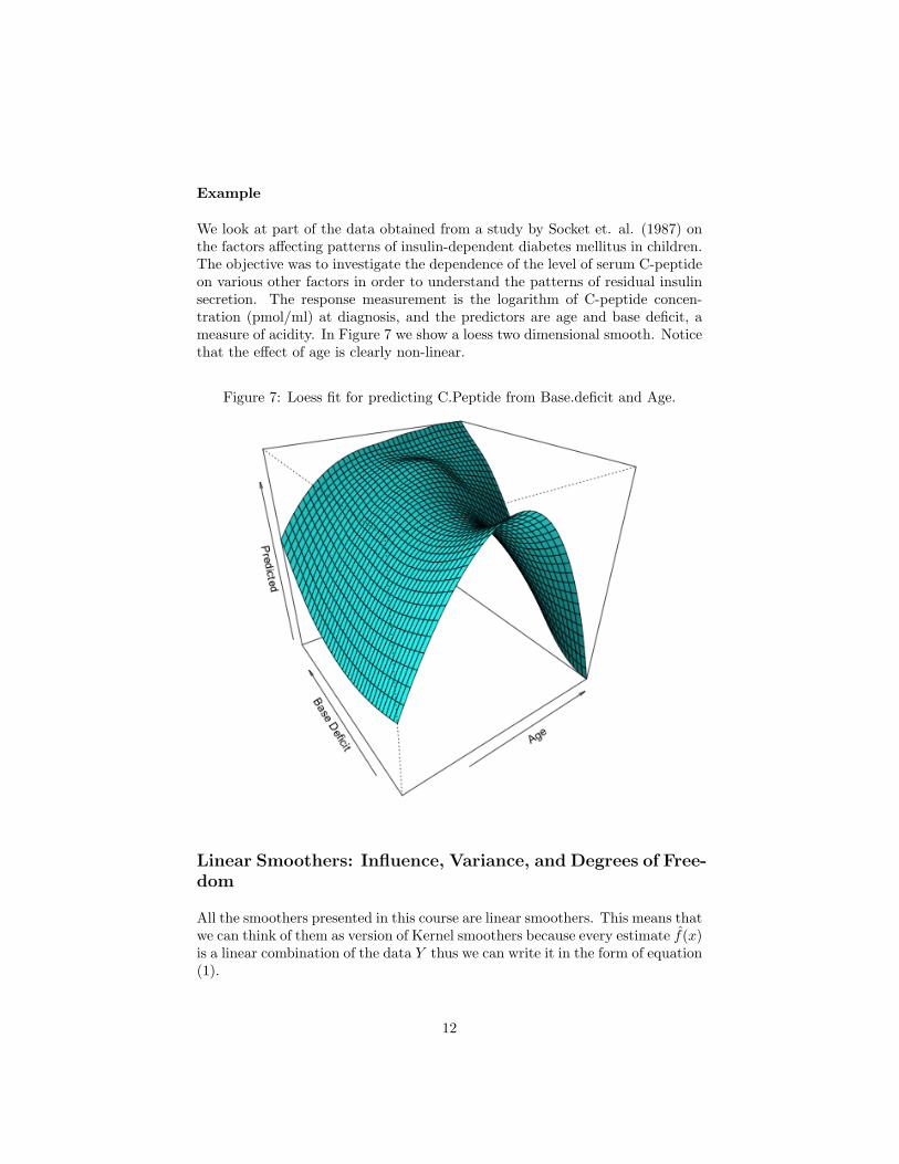
We look at part of the data obtained from a study by Socket et. al. (1987) onthe factors affecting patterns of insulin-dependent diabetes mellitus in children.The objective was to investigate the dependence of the level of serum C-peptideon various other factors in order to understand the patterns of residual insulinsecretion. The response measurement is the logarithm of C-peptide concen-tration (pmol/ml) at diagnosis, and the predictors are age and base deficit, ameasure of acidity. In Figure 7 we show a loess two dimensional smooth. Noticethat the effect of age is clearly non-linear.

Figure 7: Loess fit for predicting C.Peptide from Base.deficit and Age.

Linear Smoothers: Influence, Variance, and Degrees of Free-dom

All the smoothers presented in this course are linear smoothers. This means thatwe can think of them as version of Kernel smoothers because every estimate f(x)is a linear combination of the data Y thus we can write it in the form of equation(1).

12

If we forget about estimating f at every possible x and consider only the ob-serverd (or design) points x1, . . . , xn, we can write equation (1) as

f = Sy.

Here f = f(x1), . . . , f(xn) and S is defined by the algorithm we are using.

Question: What is S for linear regression? How about for the kernel smootherdefined above?

How can we characterize the amount of smoothing being performed? Thesmoothing parameters provide a characterization, but it is not ideal because itdoes not permit us to compare between different smoothers and for smootherslike loess it does not take into account the shape of the weight function nor thedegree of the polynomial being fit.

We now use the connections between smoothing and multivariate linear regres-sion (they are both linear smoothers) to characterize pointwise criteria thatcharacterize the amount of smoothing at a single point and global criteria thatcharacterize the global amount of smoothing.

We will define variance reduction, influence, and degrees of freedom for linearsmoothers.

The variance of the interpolation estimate is var[Y1] = σ2. The variance of oursmooth estimate is

var[f(x)] = σ2n∑

i=1

W 2i (x)

so we define∑n

i=1W2i (x) as the variance reduction. Under mild conditions one

can show that this is less than 1.

Becausen∑

i=1

var[f(xi)] = tr(SS′)σ2,

the total variance reduction from∑n

i=1 var[Yi] is tr(SS′)/n.

In linear regression the variance reduction is related to the degrees of freedom,or number of parameters. For linear regression,

∑ni=1 var[f(xi)] = pσ2. One

widely used definition of degrees of freedoms for smoothers is df = tr(SS′).

The sensitivity of the fitted value, say f(xi), to the data point yi can be mea-sured by Wi(xi)/

∑ni=1Wn(xi) or Sii (remember the denominator is usually

1).

The total influence or sensitivity is∑n

i=1Wi(xi) = tr(S).

In linear regression tr(S) = p is also equivalent to the degrees of freedom. Thisis also used as a definition of degrees of freedom.

13

Figure 8: Degrees of freedom for loess and smoothing splines as functions of thesmoothing parameter. We define smoothing splines in a later lecture.

Finally we notice that

E[(y − f)′(y − f)] = n− 2tr(S) + tr(SS′)σ2

In the linear regression case this is (n− p)σ2. We therefore denote n− 2tr(S) +tr(SS′) as the residual degrees of freedom. A third definition of degrees offreedom of a smoother is then 2tr(S)− tr(SS′).

Under relatively mild assumptions we can show that

1 ≤ tr(SS′) ≤ tr(S) ≤ 2tr(S)− tr(SS′) ≤ n

Splines and Friends: Basis Expansion and Regularization

Through-out this section, the regression function f will depend on a single, real-valued predictor X ranging over some possibly infinite interval of the real line,I ⊂ R. Therefore, the (mean) dependence of Y on X is given by

f(x) = E(Y |X = x), x ∈ I ⊂ R. (3)

For spline models, estimate definitions and their properties are more easily char-acterized in the context of linear spaces.

Linear Spaces

In this chapter our approach to estimating f involves the use of finite dimen-sional linear spaces.

14

Figure 9: Comparison of three definition of degrees of freedom

Remember what a linear space is? Remember definitions of dimension, linearsubspace, orthogonal projection, etc. . .

Why use linear spaces?

• Makes estimation and statistical computations easy.

• Has nice geometrical interpretation.

• It actually can specify a broad range of models given we have discretedata.

Using linear spaces we can define many families of function f ; straight lines,polynomials, splines, and many other spaces (these are examples for the casewhere x is a scalar). The point is: we have many options.

Notice that in most practical situation we will have observations (Xi, Yi), i =1, . . . , n. In some situations we are only interested in estimating f(Xi), i =1, . . . , n. In fact, in many situations it is all that matters from a statisticalpoint of view. We will write f when referring to the this vector and f whenreferring to an estimate. Think of how its different to know f and know f .

15

Let’s say we are interested in estimating f . A common practice in statistics isto assume that f lies in some linear space, or is well approximated by a g thatlies in some linear space.

For example for simple linear regression we assume that f lies in the linear spaceof lines:

α+ βx, (α, β)′ ∈ R2.

For linear regression in general we assume that f lies in the linear space of linearcombinations of the covariates or rows of the design matrix. How do we writeit out?

Note: Through out this chapter f is used to denote the true regression functionand g is used to denote an arbitrary function in a particular space of functions.It isn’t necessarily true that f lies in this space of function. Similarly we use fto denote the true function evaluated at the design points or observed covariatesand g to denote an arbitrary function evaluated at the design points or observedcovariates.

Now we will see how and why it’s useful to use linear models in a more generalsetting.

Technical note: A linear model of order p for the regression function (3)consists of a p-dimensional linear space G, having as a basis the function

Bj(x), j = 1, . . . , p

defined for x ∈ I. Each member g ∈ G can be written uniquely as a linearcombination

g(x) = g(x; θ) = θ1B1(x) + · · ·+ θpBp(x)

for some value of the coefficient vector θ = (θ1, . . . , θp)′ ∈ Rp.

Notice that θ specifies the point g ∈ G.

How would you write this out for linear regression?

Given observations (Xi, Yi), i = 1, . . . , n the least squares estimate (LSE) of for equivalently f(x) is defined by f(x) = g(x; θ), where

θ = arg minθ∈Rp

n∑i=1

Yi − g(Xi,θ)2.

Define the vector g = g(x1), . . . , g(xn)′. Then the distribution of the obser-vations of Y |X = x are in the family

N(g, σ2In); g = [g(x1), . . . , g(xn)]′, g ∈ G (4)

and if we assume the errors ε are IID normal and that f ∈ G we have thatf = [g(x1; θ), . . . , g(xn; θ)] is the

16

maximum likelihood estimate. The estimand f is an n × 1 vector. But howmany parameters are we really estimating?

Equivalently we can think of the distribution is in the family

N(Bθ, σ2); θ ∈ Rp (5)

and the maximum likelihood estimate for θ is θ. Here B is a matrix of basiselements defined soon. . .

Here we start seeing for the first time where the name non-parametric comesfrom. How are the approaches (4) and (5) different?

Notice that obtaining θ is easy because of the linear model set-up. The ordinaryleast square estimate is

(B′B)θ = B′Y

where B is is the n × p design matrix with elements [B]ij = Bj(Xi). Whenthis solution is unique we refer to g(x; θ) as the OLS projection of Y into G (aslearned in the first term).

Parametric versus non-parametric

In some cases, we have reason to believe that the function f is actually a memberof some linear space G. Traditionally, inference for regression models dependson f being representable as some combination of known predictors. Under thisassumption, f can be written as a combination of basis elements for some valueof the coefficient vector θ. This provides a parametric specification for f . Nomatter how many observations we collect, there is no need to look outside thefixed, finite-dimensional, linear space G when estimating f .

In practical situations, however, we would rarely believe such relationship to beexactly true. Model spaces G are understood to provide (at best) approximationsto f ; and as we collect more and more samples, we have the freedom to auditionricher and richer classes of models. In such cases, all we might be willing tosay about f is that it is smooth in some sense, a common assumption beingthat f have two bounded derivatives. Far from the assumption that f belongto a fixed, finite-dimensional linear space, we instead posit a nonparametricspecification for f . In this context, model spaces are employed mainly in ourapproach to inference; first in the questions we pose about an estimate, andthen in the tools we apply to address them. For example, we are less interestedin the actual values of the coefficient θ, e.g. whether or not an element of θ issignificantly different from zero to the 0.05 level. Instead we concern ourselveswith functional properties of g(x; θ), the estimated curve or surface, e.g. whetheror not a peak is real.

To ascertain the local behavior of OLS projections onto approximation spacesG, define the pointwise, mean squared error (MSE) of g(x) = g(x; θ) as

Ef(x)− g(x)2 = bias2g(x)+ varg(x)

17

wherebiasg(x) = f(x)− Eg(x) (6)

andvarg(x) = Eg(x)− E[g(x)]2

When the input values Xi are deterministic the expectations above are withrespect to the noisy observation Yi. In practice, MSE is defined in this way evenin the random design case, so we look at expectations conditioned on X.

Note: The MSE and EPE are equivalent. The only difference is that we ignorethe first σ2 due to measuremnet error contained in the EPE. The reason I useMSE here is because it is what is used in the Spline and Wavelet literature.

When we do this, standard results in regression theory can be applied to derivean expression for the variance term

varg(x) = σ2B(x)′(B′B)−1B(x)

where B(x) = (B1(x), . . . , Bp(x))′, and the error variance is assumed constant.

Under the parametric specification thatf ∈ G, what is the bias?

This leads to classical t- and F-hypothesis tests and associated parametric con-fidence intervals for θ. Suppose on the other hand, that f is not a member ofG, but rather can be reasonably approximated by an element in G. The bias (6)now reflects the ability of functions in G to capture the essential features of f .

Local Polynomials

In practical situations, a statistician is rarely blessed with simple linear rela-tionship between the predictor X and the observed output Y . That is, as adescription of the regression function f , the model

g(x; θ) = θ1 + θ2x, x ∈ I

typically ignores obvious features in the data. This is certainly the case for thevalues of 87Sr.

The Strontium data set was collected to test several hypotheses about the catas-trophic events that occurred approximately 65 million years ago. The data con-tains Age in million of years and the ratios described here. There is a divisionbetween two geological time periods, the Cretaceous (from 66.4 to 144 millionyears ago) and the Tertiary (spanning from about 1.6 to 66.4 million years ago).Earth scientist believe that the boundary between these periods is distinguishedby tremendous changes in climate that accompanied a mass extension of overhalf of the species inhabiting the planet at the time. Recently, the composi-tions of Strontium (Sr) isotopes in sea water has been used to evaluate several

18

hypotheses about the cause of these extreme events. The dependent variableof the data-set is related to the isotopic make up of Sr measured for the shellsof marine organisms. The Cretaceous-Tertiary boundary is referred to as KTB.There data shows a peak is at this time and this is used as evidence that ameteor collided with earth.

The data presented in the Figure ?? represents standardized ratio of strontium–87 isotopes (87Sr) to strontium–86 isotopes (86Sr) contained in the shells offoraminifera fossils taken form cores collected by deep sea drilling. For eachsample its time in history is computed and the standardized ratio is computed:

87δSr =(

87Sr/86Sr sample87Sr/86Sr sea water

− 1)× 105.

Earth scientist expect that 87δSr is a smooth-varying function of time and thatdeviations from smoothness are mostly measurement error.

Figure 10: 87δSr data.

To overcome this deficiency, we might consider a more flexible polynomial model.

19

Let Pk denote the linear space of polynomials in x of order at most k defined as

g(x; θ) = θ1 + θ2x+ · · ·+ θkxk−1, x ∈ I

for the parameter vector θ = (θ1, . . . , θk) ∈ Rk. Note that the space Pk consistsof polynomials having degree at most k − 1.

In exceptional cases, we have reasons to believe that the regression function fis in fact a high-order polynomial. This parametric assumption could be basedon physical or physiological models describing how the data were generated.

For historical values of 87δSr we consider polynomials simply because our sci-entific intuition tells us that f should be smooth.

Recall Taylor’s theorem: polynomials are good at approximating well-behavedfunctions in reasonably tight neighborhoods. If all we can say about f is thatit is smooth in some sense, then either implicitly or explicitly we consider high-order polynomials because of their favorable approximation properties.

If f is not in Pk then our estimates will be biased by an amount that reflectsthe approximation error incurred by a polynomial model.

Computational Issue: The basis of monomials

Bj(x) = xj−1 for j = 1, . . . , k

is not well suited for numerical calculations (x8 can be VERY BIG compared tox). While convenient for analytical manipulations (differentiation, integration),this basis is ill-conditioned for k larger than 8 or 9. Most statistical packagesuse the orthogonal Chebyshev polynomials (used by the R command poly()).

An alternative to polynomials is to consider the space PPk(t) of piecewisepolynomials with break points t = (t0, . . . , tm+1)′. Given a sequence a = t0 <t1 < · · · < tm < tm+1 = b, construct m+ 1 (disjoint) intervals

Il = [tl−1, tl), 1 ≤ l ≤ m and Im+1 = [tm, tm+1],

whose union is I = [a, b]. Define the piecewise polynomials of order k

g(x) =

g1(x) = θ1,1 + θ1,2x+ · · ·+ θ1,kx

k−1, x ∈ I1...

...gm+1(x) = θm+1,1 + θm+1,2x+ · · ·+ θm+1,kx

k−1, x ∈ Ik+1.

Splines

In many situations, breakpoints in the regression function do not make sense.Would forcing the piecewise polynomials to be continuous suffice? What aboutcontinuous first derivatives?

20

We start by consider the subspaces of the piecewise polynomial space. We willdenote it with PPk(t) with t = (t1, . . . , tm)′ the break-points or interior knots.Different break points define different spaces.

We can put constrains on the behavior of the functions g at the break points.(We can construct tests to see if these constrains are suggested by the data but,will not go into this here)

Here is a trick for forcing the constrains and keeping the linear model set-up.We can write any function g ∈ PPk(t) in the truncated basis power :

g(x) = θ0,1 + θ0,2x+ · · ·+ θ0,kxk−1 +

θ1,1(x− t1)0+ + θ1,2(x− t1)1+ + · · ·+ θ1,k(x− t1)k−1+ +

...θm,1(x− tm)0+ + θm,2(x− tm)1+ + · · ·+ θm,k(x− tm)k−1

+

where (·)+ = max(·, 0). Written in this way the coefficients θ1,1, . . . , θ1,k recordthe jumps in the different derivative from the first piece to the second.

Notice that the constrains reduce the number of parameters. This is in agree-ment with the fact that we are forcing more smoothness.

Now we can force constrains, such as continuity, by putting constrains likeθ1,1 = 0 etc. . .

We will concentrate on the cubic splines which are continuous and have contin-uous first and second derivatives. In this case we can write:

g(x) = θ0,1 + θ0,2x+ · · ·+ θ0,4x3 + θ1,k(x− t1)3 + · · ·+ θm,k(x− tm)3

How many “parameters” in this space?

Note: It is always possible to have less restrictions at knots where we believe thebehavior is “less smooth”, e.g for the Sr ratios, we may have “unsmoothness”around KTB.

We can write this as a linear space. This setting is not computationally conve-nient. In S-Plus there is a function bs() that makes a basis that is convenientfor computations.

There is asymptotic theory that goes along with all this but we will not go intothe details. We will just notice that

E[f(x)− g(x)] = O(h2kl + 1/nl)

where hl is the size of the interval where x is in and nl is the number of pointsin it. What does this say?

21

Splines in terms of Spaces and sub-spaces

The p-dimensional spaces described in Section 4.1 were defined through basisfunction Bj(x), j = 1, . . . , p. So in general we defined for a given range I ⊂ Rk

G = g : g(x) =p∑

j=1

θjβj(x),x ∈ I, (θ1, . . . , θp) ∈ Rp

In the previous section we concentrated on x ∈ R.

In practice we have design points x1, . . . , xn and a vector of responses y =(y1, . . . , yn). We can think of y as an element in the n-dimensional vector spaceRn. In fact we can go a step further and define a Hilbert space with the usualinner product definition that gives us the norm

||y|| =n∑

i=1

y2i

Now we can think of least squares estimation as the projection of the data y tothe sub-space G ⊂ Rn defined by G in the following way

G = g ∈ Rn : g = [g(x1), . . . , g(xn)]′, g ∈ G

Because this space is spanned by the vectors [B1(x1), . . . , Bp(xn)] the projectionof y onto G is

B(B′B)−B′y

as learned in 751. Here [B]ij = Bj(xi).

Natural Smoothing Splines

Natural splines add the constrain that the function must be linear after theknots at the end points. This forces 2 more restrictions since f ′′ must be 0 atthe end points, i.e the space has k + 4 − 2 parameters because of this extra 2constrains.

So where do we put the knots? How many do we use? There are some data-driven procedures for doing this. Natural Smoothing Splines provide anotherapproach.

What happens if the knots coincide with the dependent variables Xi. Thenthere is a function g ∈ G, the space of cubic splines with knots at (x1, . . . , xn),with g(xi) = yi, i, . . . , n, i.e. we haven’t smoothed at all.

Consider the following problem: among all functions g with two continuous firsttwo derivatives, find one that minimizes the penalized residual sum of squares

n∑i=1

yi − g(xi)2 + λ

∫ b

a

g′′(t)2 dt

22

where λ is a fixed constant, and a ≤ x1 ≤ · · · ≤ xn ≤ b. It can be shown(Reinsch 1967) that the solution to this problem is a natural cubic spline withknots at the values of xi (so there are n− 2 interior knots and n− 1 intervals).Here a and b are arbitrary as long as they contain the data.

It seems that this procedure is over-parameterized since a natural cubic splineas this one will have n degrees of freedom. However we will see that the penaltymakes this go down.

Computational Aspects

We use the fact that the solution is a natural cubic spline and write the possibleanswers as

g(x) =n∑

j=1

θjBj(x)

where θj are the coefficients and Bj(x) are the basis functions. Notice that ifthese were cubic splines the functions lie in a n+ 2 dimensional space, but thenatural splines are an n dimensional subspace.

Let B be the n× n matrix defined by

Bij = Bj(xi)

and a penalty matrix Ω by

Ωij =∫ b

a

B′′i (t)B′′j (t) dt

now we can write the penalized criterion as

(y −Bθ)′(y −Bθ) + λθ′Ωθ

It seems there are no boundary derivatives constraints but they are implicitlyimposed by the penalty term.

Setting derivatives with respect to θ equal to 0 gives the estimating equation:

(B′B + λΩ)θ = B′y.

The θ that solves this equation will give us the estimate g = Bθ.

Is this a linear smoother?

Write:g = Bθ = B(B′B + λΩ)−1B′y = (I + λK)−1y

where K = B− 1′ΩB−1. Notice we can write the criterion as

(y − g)′(y − g) + λg′Kg

If we look at the “kernel” of this linear smoother we will see that it is similarto the other smoothers presented in this class.

23

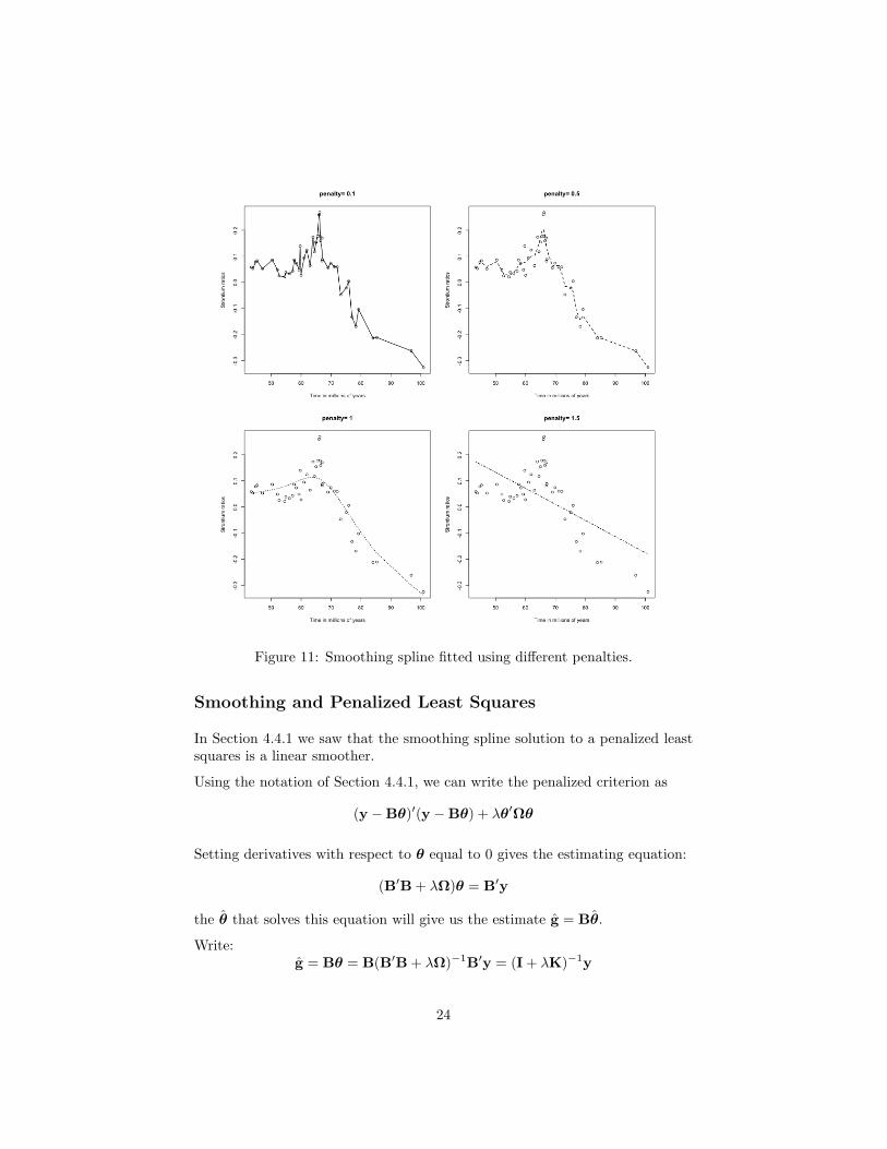
Figure 11: Smoothing spline fitted using different penalties.

Smoothing and Penalized Least Squares

In Section 4.4.1 we saw that the smoothing spline solution to a penalized leastsquares is a linear smoother.

Using the notation of Section 4.4.1, we can write the penalized criterion as

(y −Bθ)′(y −Bθ) + λθ′Ωθ

Setting derivatives with respect to θ equal to 0 gives the estimating equation:

(B′B + λΩ)θ = B′y

the θ that solves this equation will give us the estimate g = Bθ.

Write:g = Bθ = B(B′B + λΩ)−1B′y = (I + λK)−1y

24

where K = B′−ΩB−.

Notice we can write the penalized criterion as

(y − g)′(y − g) + λg′Kg

If we plot the rows of this linear smoother we will see that it is like a kernelsmoother.

Figure 12: Kernels of a smoothing spline.

Notice that for any linear smoother with a symmetric and nonnegative definiteS, i.e. there S− exists, then we can argue in reverse: f = Sy is the value thatminimizes the penalized least squares criteria of the form

(y − f)′(y − f) + f ′(S− − I)f .

Some of the smoothers presented in this class are not symmetrical but are close.In fact for many of them one can show that asymptotically they are symmetric.

Eigen analysis and spectral smoothing

For a smoother with symmetric smoother matrix S, the eigendecomposition ofS can be used to describe its behavior.

25

Let u1, . . . ,un be an orthonormal basis of eigenvectors of S with eigenvaluesθ1 ≥ θ2 · · · ≥ θn:

Suj = θjuj , j = 1, . . . , n

or

S = UDU′ =n∑

j=1

θjuju′j .

Here D is a diagonal matrix with the eigenvalues as the entries.

For simple linear regression we only have two nonzero eigenvalues. Their eigen-vectors are an orthonormal basis for lines.

Figure 13: Eigenvalues and eigenvectors of the hat matrix for linear regression.

The cubic spline is an important example of a symmetric smoother, and itseigenvectors resemble polynomials of increasing degree.

It is easy to show that the first two eigenvalues are unity, with eigenvectorswhich correspond to linear functions of the predictor on which the smoother isbased. One can also show that the other eigenvalues are all strictly betweenzero and one.

The action of the smoother is now transparent: if presented with a responsey = uj , it shrinks it by an amount θj as above.

26

Figure 14: Eigenvalues and eigenvectors 1 through 10 of S for a smoothingspline.

Cubic smoothing splines, regression splines, linear regression, polynomial regres-sion are all symmetric smoothers. However, loess and other “nearest neighbor”smoothers are not.

Figure 15: Eigen vectors 11 through 30 for a smoothing spline for n = 30.

If S is not symmetric we have complex eigenvalues and the above decompositionis not as easy to interpret. However we can use the singular value decomposition

S = UDV′

On can think of smoothing as performing a basis transformation z = V′y,shrinking with z = Dz the components that are related to “unsmooth compo-nents” and then transforming back to the basis y = Uz we started out with. . .sort of.

27

In signal processing signals are “filtered” using linear transformations. Thetransfer function describes how the power of certain frequency components arereduced. A low-pass filter will reduce the power of the higher frequency com-ponents. We can view the eigen values of our smoother matrices as transferfunctions.

Notice that the smoothing spline can be considered a low-pass filter. If welook at the eigenvectors of the smoothing spline we notice they are similar tosinusoidal components of increasing frequency. Figure 14 shows the “transferfunction” defined by the smoothing splines.

Economical Bases: Wavelets and REACT estimators

If one consider the “equally spaced” Gaussian regression:

yi = f(ti) + εi, i = 1, . . . , n (7)

ti = (i− 1)/n and the εis IID N(0, σ2), many things simplify.

We can write this in matrix notation: the response vector y is Nn(f , σ2I) withf = f(t1), . . . , f(tn)′.

As usual we want to find an estimation procedure that minimizes risk:

n−1E||f − f ||2 = n−1E

[m∑

i=1

f(ti)− f(ti)2].

We have seen that the MLE is fi = yi which intuitively does not seem veryuseful. There is actually animportant result in statistics that makes this more precise.

Stein (1956) noticed that the MLE is inadmissible: There is an estimationprocedure producing estimates with smaller risk that the MLE for any f .

To develop a non-trivial theory MLE won’t do. A popular procedure is to spec-ify some fixed class F of functions where f lies and seek an estimator f attainingminimax risk

inff

supf∈F

R(f , f)

By restricting f ∈ F we make assumptions on the smoothness of f . For example,the L2 Sobolev family makes an assumption on the number m of continuousderivatives and a limits the size of the mth derivative.

28

Useful transformations

Remember f ∈ Rn and that there are many orthogonal bases for this space.Any orthogonal basis can be represented with an orthogonal transform U thatgives us the coefficients for any f by multiplying ξ = U′f . This means that wecan represent any vector as f = Uξ.

Remember that the eigen analysis of smoothing splines we can view the eigen-vectors a such a transformation.

If we are smart, we can choose a transformation U such that ξ has some usefulinterpretation. Furthermore, certain transformation may be more “economical”as we will see.

For equally spaced data a widely used transformation is the Discrete FourierTransform (DFT). Fourier’s theorem says that any f ∈ Rn

can be re-written as

fi = a0 +n/2−1∑k=1

ak cos

(2πkn

i

)+ bk sin

(2πkn

i

)+ an/2 cos(πi)

for i = 1, . . . , n. This defines a basis and the coefficients a = (a0, a1, b1, . . . , . . . , an/2)′

can be obtained via a = U′f with U having columns of sines and cosines:

U1 = [n−1/2 : 1 ≤ i ≤ n]U2k = [(2/n)1/2 sin2πki/n : 1 ≤ i ≤ n], k = 1, . . . , n/2

U2k+1 = [(2/n)1/2 cos2πki/n : 1 ≤ i ≤ n], k = 1, . . . , n/2− 1.

Note: This can easily be changed to the case where n is odd by substitutingn/2 by bn/2c and taking out the last term last term adn/2e.

If a signal is close to a sine wave f(t) = cos(2πjt/n + φ) for some integer1 ≤ j ≤ n, only two of the coefficients in a will be big, namely the onesassociated with the columns 2j − 1 and 2j, the rest will be close to 0.

This makes the basis associated with the DFT very economical (and the peri-odogram a good detector of hidden periodicities). Consider that if we whereto transmit the signal, say using modems and a telephone line, it would bemore “economical” to send a instead of the f . Once a is received, f = Ua isreconstructed. This is basically what data compression is all about.

Because we are dealing with equally spaced data, the coefficients of the DFTare also related to smoothness. Notice that the columns of U are increasing infrequency and thus decreasing in smoothness. This means that a “smooth” fshould have only the first a = U′f relatively different from 0.

A close relative of the DFT is the Discrete Cosine Transform (DCT).

U1 = [n−1/2 : 1 ≤ i ≤ n]Uk = [(2/n)1/2 cosπ(2i− 1)k/(2/n) : 1 ≤ i ≤ n], k = 2, . . . , n

29

Economical bases together with “shrinkage” ideas can be used to reduce riskand even to obtain estimates with minimax properties. We will see this throughan example

An example

We consider body temperature data taken from a mouse every 30 minutes fora day, so we have n = 48. We believe measurements will havemeasurement error and maybe environmental variability so we use a stochasticmodel like (7). We expect body temperature to change “smoothly” through-outthe day so we believe f(x) is smooth. Under this assumption ξ = U′f , with Uthe DCT, should have only a few coefficients that are “big”.

Because the transformation is orthogonal we have that z = U′y is N(ξ, σ2I).An idea we learn from Stein (1956) is to consider linear shrunken estimatesξ = wz; w ∈ [0, 1]n. Here the product wz is taken component-wise like inS-plus.

We can then choose the shrinkage coefficients that minimize the risk

E||ξ − ξ||2 = E||Uξ − f ||2.

30

Remember that Uξ = UU′f = f .

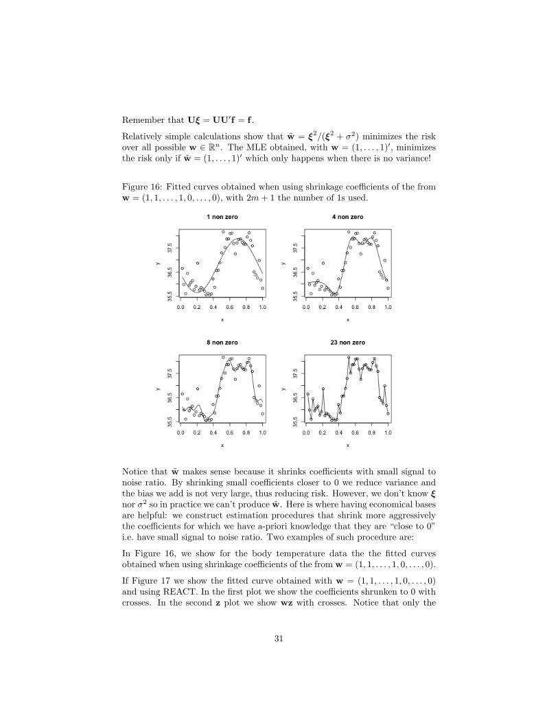
Relatively simple calculations show that w = ξ2/(ξ2 + σ2) minimizes the riskover all possible w ∈ Rn. The MLE obtained, with w = (1, . . . , 1)′, minimizesthe risk only if w = (1, . . . , 1)′ which only happens when there is no variance!

Figure 16: Fitted curves obtained when using shrinkage coefficients of the fromw = (1, 1, . . . , 1, 0, . . . , 0), with 2m+ 1 the number of 1s used.

Notice that w makes sense because it shrinks coefficients with small signal tonoise ratio. By shrinking small coefficients closer to 0 we reduce variance andthe bias we add is not very large, thus reducing risk. However, we don’t know ξnor σ2 so in practice we can’t produce w. Here is where having economical basesare helpful: we construct estimation procedures that shrink more aggressivelythe coefficients for which we have a-priori knowledge that they are “close to 0”i.e. have small signal to noise ratio. Two examples of such procedure are:

In Figure 16, we show for the body temperature data the the fitted curvesobtained when using shrinkage coefficients of the from w = (1, 1, . . . , 1, 0, . . . , 0).

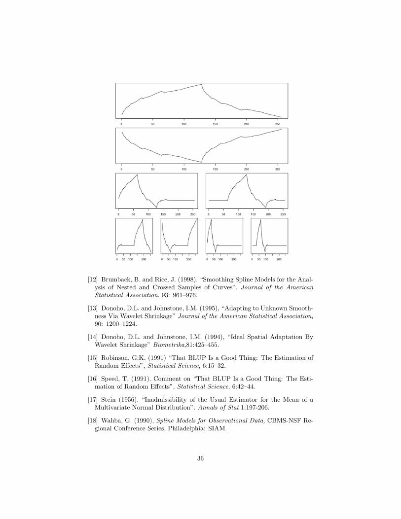
If Figure 17 we show the fitted curve obtained with w = (1, 1, . . . , 1, 0, . . . , 0)and using REACT. In the first plot we show the coefficients shrunken to 0 withcrosses. In the second z plot we show wz with crosses. Notice that only the

31

Figure 17: Estimates obtained with harmonic model and with REACT. We alsoshow the z and how they have been shrunken.

first few coefficients of the transformation are “big”. Here are the same picturesfor data obtained for 6 consecutive weekends.

Finally in Figure 18 we show the two fitted curves and compare them to theaverage obtained from observing many days of data.

Notice that using w = (1, 1, 1, 1, 0, . . . , 0) reduces to a parametric model thatassumes f is a sum of 4 cosine functions.

Any smoother with a smoothing matrix S that is a projection, e.g. linear re-gression, splines, can be consider a special case of what we have described here.

Choosing the transformation U is an important step in these procedure. Thetheory developed for Wavelets motivate a choice of U that is especially good athandling functions f that have “discontinuities”.

Wavelets

The following plot show a nuclear magnetic resonance (NMR) signal.

32

Figure 18: Comparison of two fitted curves to the average obtained from ob-serving many days of data.

The signal does appear to have some added noise so we could use (7) to modelthe process. However, f(x) appears to have a peak at around x = 500 makingit not very smooth at that point.

Situations like these are where wavelets analyses is especially useful for “smooth-ing”. Now a more appropriate word is “de-noising”.

The Discrete Wavelet Transform defines an orthogonal basis just like the DFTand DCT. However the columns of DWT are locally smooth. This means thatthe coefficients can be interpreted as local smoothness of the signal for differentlocations.

Here are the columns of the Haar DWT, the simplest wavelet.

Notice that these are step function. However, there are ways (they involvecomplicated math and no closed forms) to create “smoother” wavelets. Thefollowing are the columns of DWT using the Daubechies wavelets

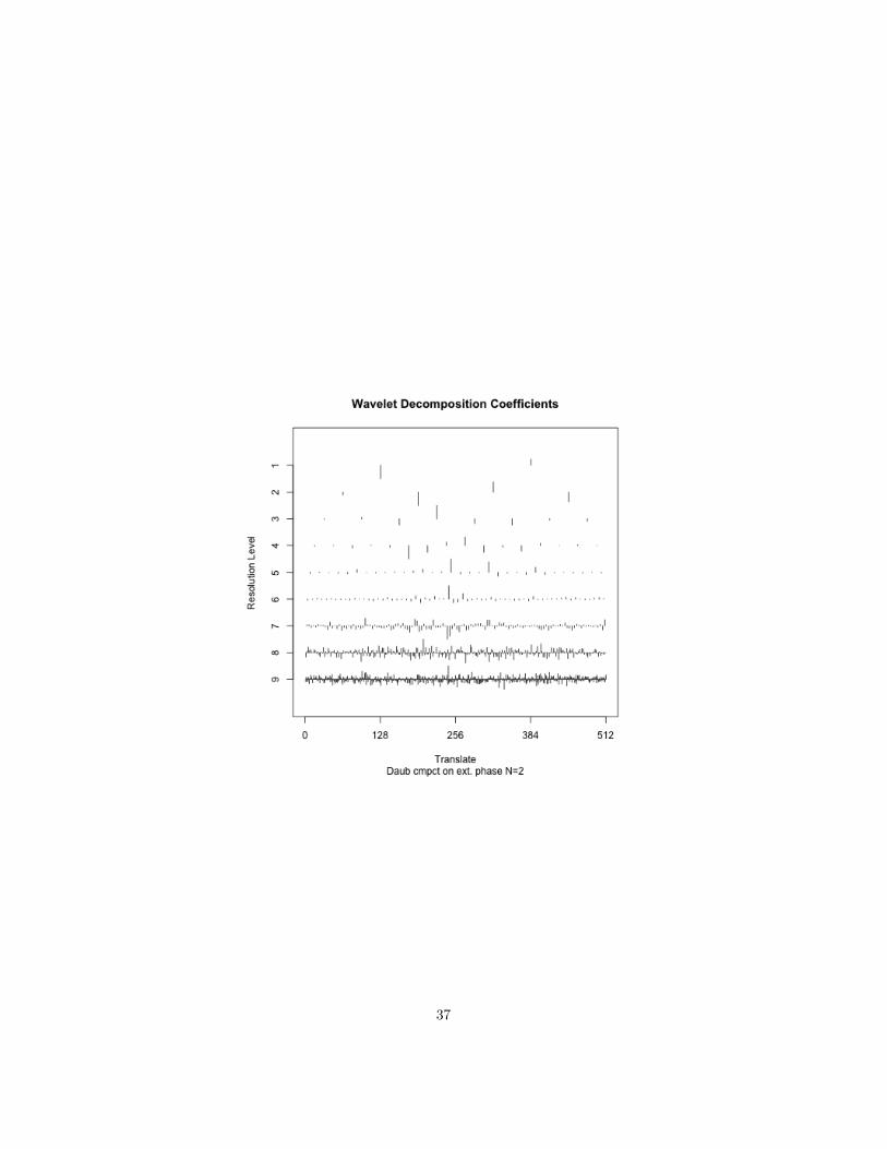
The following plot shows the coefficients of the DWT by smoothness level andby location:

33

Using wavelet with shrinkage seems to perform better at de-noising than smooth-ing splines and loess as shown by the following figure.

The last plot is what the wavelet estimate looks like for the temperature data

References

[1] Cleveland, R. B., Cleveland, W. S., McRae, J. E., and Terpenning, I. (1990).Stl: A seasonal-trend decomposition procedure based on loess. Journal ofOfficial Statistics, 6:3–33.

[2] Cleveland, W. S. and Devlin, S. J. (1988). Locally weighted regression: Anapproach to regression analysis by local fitting. Journal of the AmericanStatistical Association, 83:596–610.

[3] Cleveland, W. S., Grosse, E., and Shyu, W. M. (1993). Local regressionmodels. In Chambers, J. M. and Hastie, T. J., editors, Statistical Models inS, chapter 8, pages 309–376. Chapman & Hall, New York.

[4] Loader, C. R. (1999), Local Regression and Likelihood, New York: Springer.

34

[5] Socket, E.B., Daneman, D. Clarson, C., and Ehrich, R.M. (1987). Factorsaffecting and patterns of residual insulin secretion during the first year of typeI (insulin dependent) diabetes mellitus in children. Diabetes 30, 453–459.

[6] Eubank, R.L. (1988), Smoothing Splines and Nonparametric Regression,New York: Marcel Decker.

[7] Reinsch, C.H. (1967) Smoothing by Spline Functions. Numerische Mathe-matik, 10: 177–183

[8] Schoenberg, I.J. (1964), “Spline functions and the problem of graduation,”Proceedings of the National Academy of Science, USA 52, 947–950.

[9] Silverman (1985) “Some Aspects of the spline smoothing approach to non-parametric regression curve fitting”. Journal of the Royal Statistical SocietyB 47: 1–52.

[10] Wahba, G. (1990), Spline Models for Observational Data, CBMS-NSF Re-gional Conference Series, Philadelphia: SIAM.

[11] Beran, R. (2000). “REACT scatterplot smoothers: Superefficiency throughbasis economy”, Journal of the American Statistical Association, 95:155–171.

35

[12] Brumback, B. and Rice, J. (1998). “Smoothing Spline Models for the Anal-ysis of Nested and Crossed Samples of Curves”. Journal of the AmericanStatistical Association. 93: 961–976.

[13] Donoho, D.L. and Johnstone, I.M. (1995), “Adapting to Unknown Smooth-ness Via Wavelet Shrinkage” Journal of the American Statistical Association,90: 1200–1224.

[14] Donoho, D.L. and Johnstone, I.M. (1994), “Ideal Spatial Adaptation ByWavelet Shrinkage” Biometrika,81:425–455.

[15] Robinson, G.K. (1991) “That BLUP Is a Good Thing: The Estimation ofRandom Effects”, Statistical Science, 6:15–32.

[16] Speed, T. (1991). Comment on “That BLUP Is a Good Thing: The Esti-mation of Random Effects”, Statistical Science, 6:42–44.

[17] Stein (1956). “Inadmissibility of the Usual Estimator for the Mean of aMultivariate Normal Distribution”. Annals of Stat 1:197-206.

[18] Wahba, G. (1990), Spline Models for Observational Data, CBMS-NSF Re-gional Conference Series, Philadelphia: SIAM.

36

37

38

39