Lecture 7

Comparing Two Proportions

Let and be the two population proportions of successes. Use

to estimate .

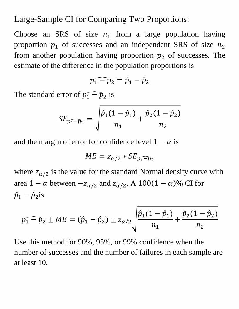
Large-Sample CI for Comparing Two Proportions:

Choose an SRS of size from a large population having

proportion of successes and an independent SRS of size

from another population having proportion of successes. The

estimate of the difference in the population proportions is

The standard error of is

√

and the margin of error for confidence level is

where is the value for the standard Normal density curve with

area between and . A CI for

is

√

Use this method for 90%, 95%, or 99% confidence when the

number of successes and the number of failures in each sample are

at least 10.

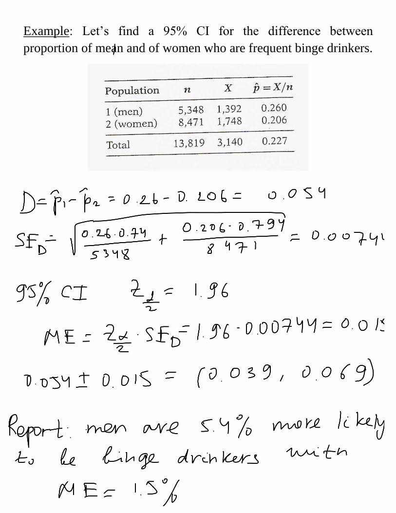
Example: Let’s find a 95% CI for the difference between

proportion of mean and of women who are frequent binge drinkers.

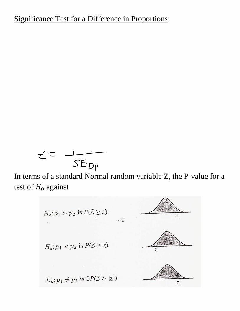
Significance Test for a Difference in Proportions:

In terms of a standard Normal random variable Z, the P-value for a

test of against

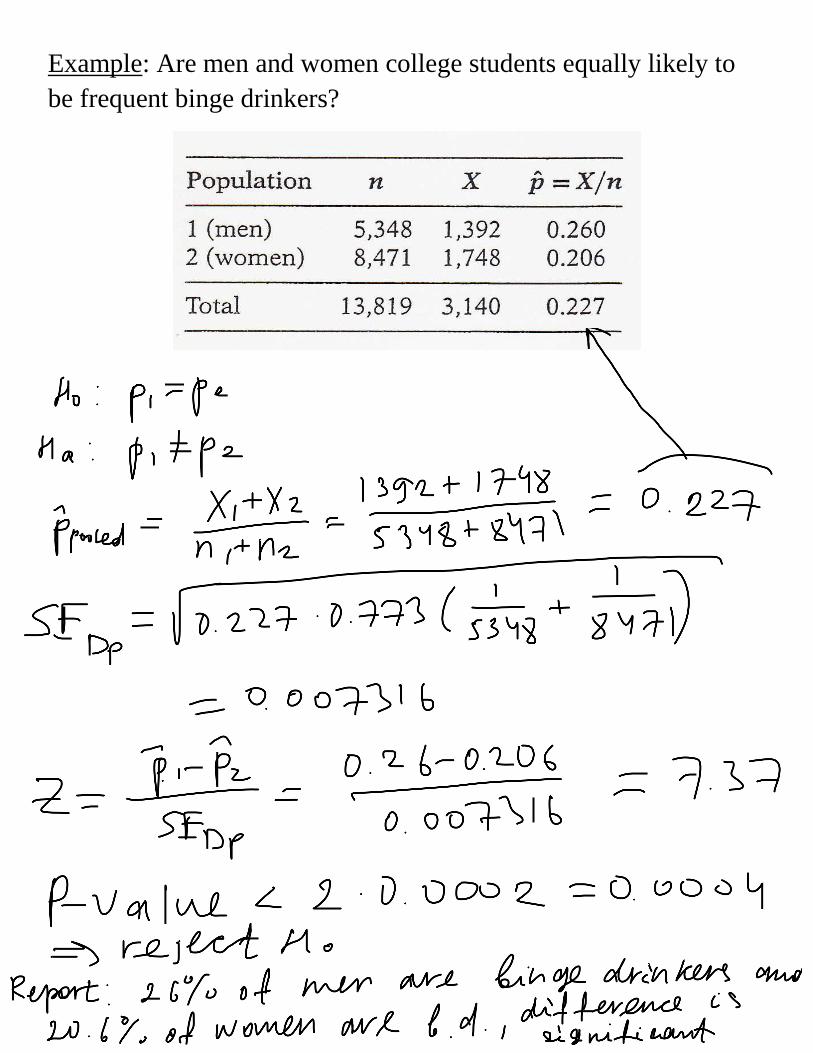
Example: Are men and women college students equally likely to

be frequent binge drinkers?

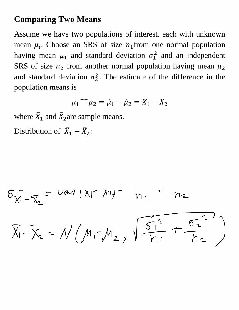
Comparing Two Means

Assume we have two populations of interest, each with unknown

mean . Choose an SRS of size from one normal population

having mean and standard deviation and an independent

SRS of size from another normal population having mean

and standard deviation . The estimate of the difference in the

population means is

where and are sample means.

Distribution of :

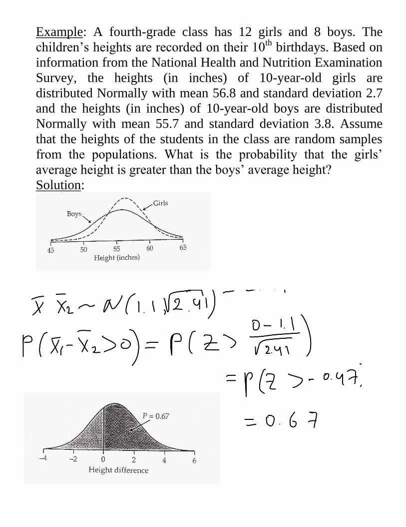
Example: A fourth-grade class has 12 girls and 8 boys. The

children’s heights are recorded on their 10th birthdays. Based on

information from the National Health and Nutrition Examination

Survey, the heights (in inches) of 10-year-old girls are

distributed Normally with mean 56.8 and standard deviation 2.7

and the heights (in inches) of 10-year-old boys are distributed

Normally with mean 55.7 and standard deviation 3.8. Assume

that the heights of the students in the class are random samples

from the populations. What is the probability that the girls’

average height is greater than the boys’ average height?

Solution:

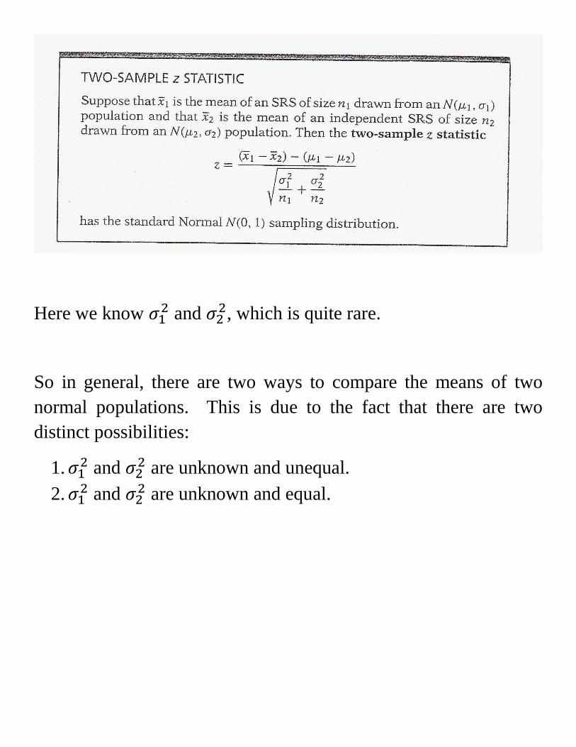
Here we know and

, which is quite rare.

So in general, there are two ways to compare the means of two

normal populations. This is due to the fact that there are two

distinct possibilities:

1. and

are unknown and unequal.

2. and

are unknown and equal.

Comparing Variances: The F Distribution

The F distribution is used to test the hypothesis that the variance of

one normal population equals the variance of another normal

population.

We shall consider

vs

(or

)

where, in the right-tailed case, denotes the larger

population variance.

The F statistic:

When and

are sample variances from independent

SRSs of sizes and drawn from Normal populations, the

F statistic

has the F distribution with and degrees of

freedom when

is true.

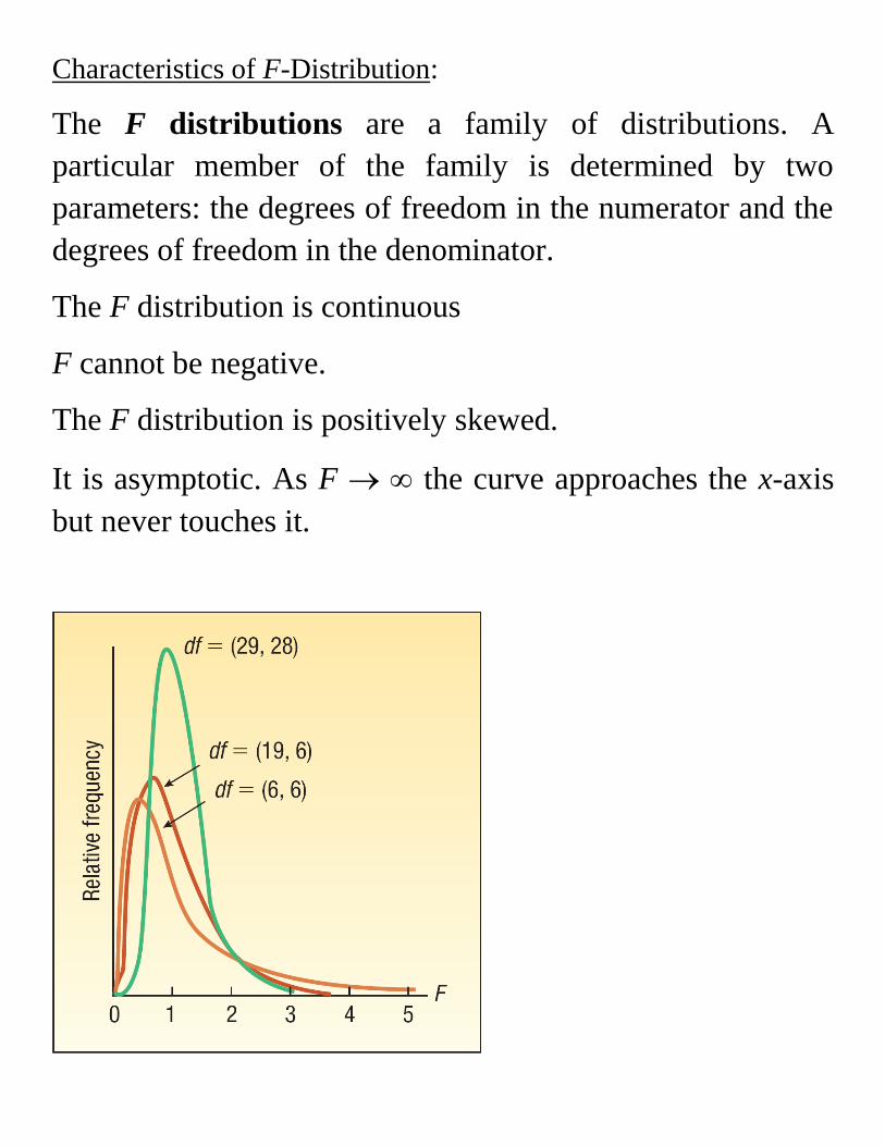
Characteristics of F-Distribution:

The F distributions are a family of distributions. A

particular member of the family is determined by two

parameters: the degrees of freedom in the numerator and the

degrees of freedom in the denominator.

The F distribution is continuous

F cannot be negative.

The F distribution is positively skewed.

It is asymptotic. As F the curve approaches the x-axis

but never touches it.

If you don’t use statistical software, arrange the F test as follows:

1. Take the test statistics to be

. This amounts to

naming the populations so that is the larger of the observed

sample variances. The resulting F is always 1 or greater.

2. Compare the value of F with the critical value from the table.

Then double the probabilities obtained from the table to get

the significance level for the two-sided F test.

Assumptions:

1. Normality is assumed, and the test is sensitive to violations of

this assumption.

2. The test for equality of variances performs best when sample

sizes are equal.

3. The test is not very powerful. To minimize this problem, it is

suggested to use a relatively high level (e.g., as high as

0.20).

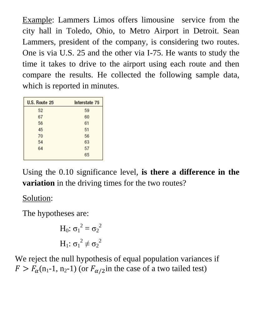
Example: Lammers Limos offers limousine service from the

city hall in Toledo, Ohio, to Metro Airport in Detroit. Sean

Lammers, president of the company, is considering two routes.

One is via U.S. 25 and the other via I-75. He wants to study the

time it takes to drive to the airport using each route and then

compare the results. He collected the following sample data,

which is reported in minutes.

Using the 0.10 significance level, is there a difference in the

variation in the driving times for the two routes?

Solution:

The hypotheses are:

H0: σ12 = σ2

2

H1: σ12 ≠ σ2

2

We reject the null hypothesis of equal population variances if

(n1-1, n2-1) (or in the case of a two tailed test)

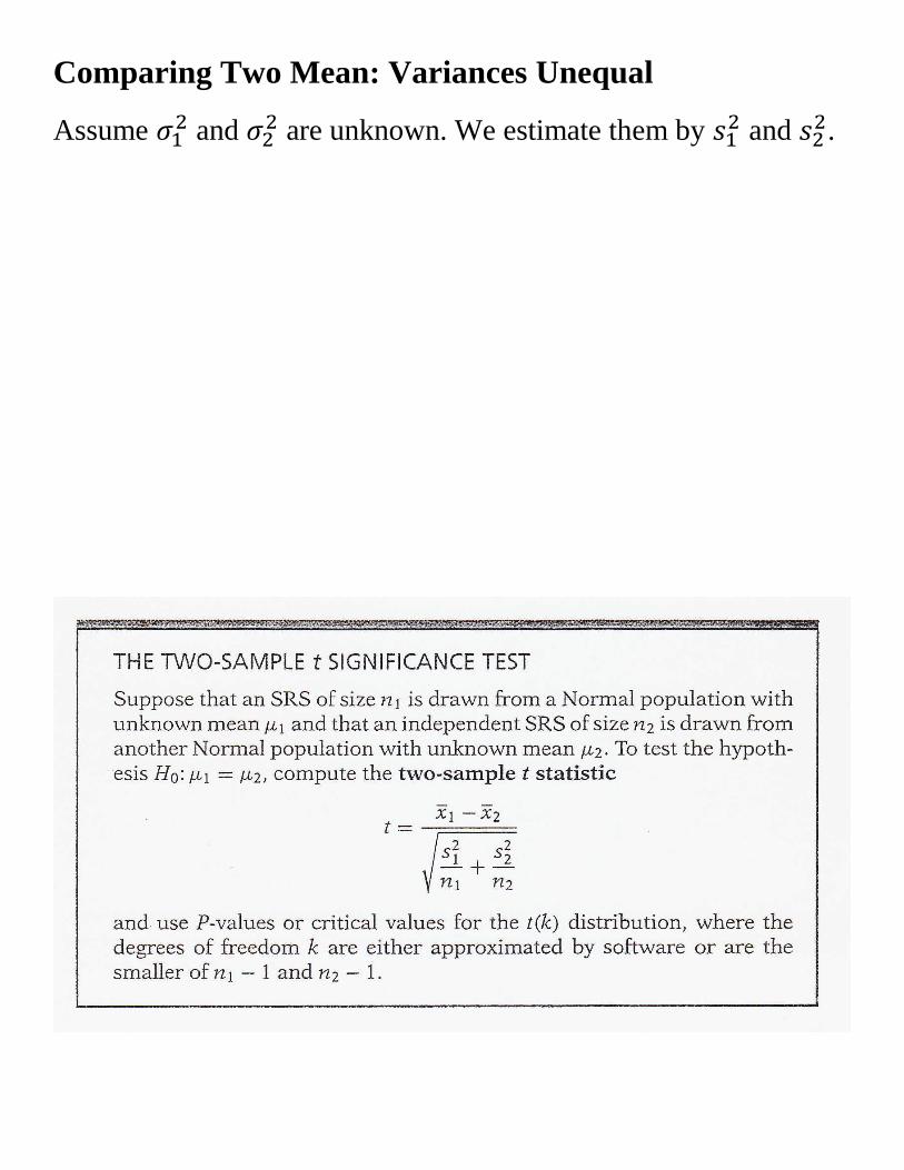
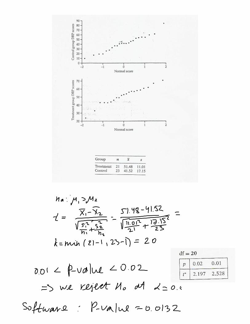
Comparing Two Mean: Variances Unequal

Assume and

are unknown. We estimate them by and

.

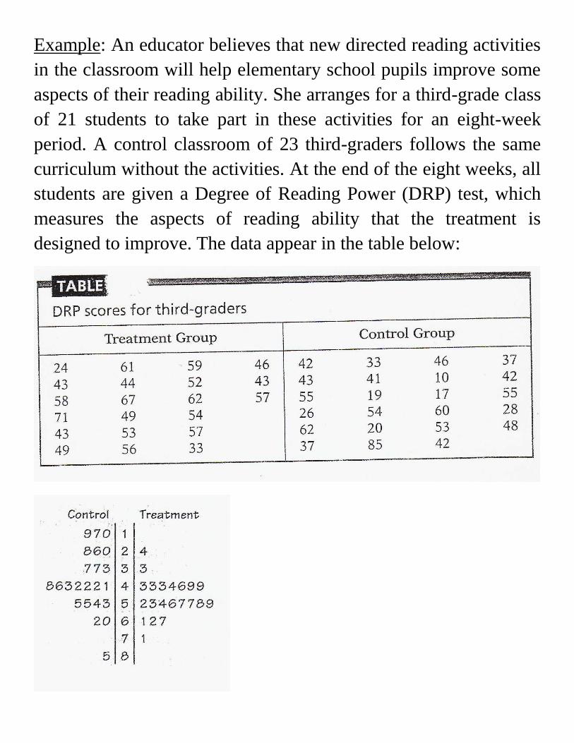
Example: An educator believes that new directed reading activities

in the classroom will help elementary school pupils improve some

aspects of their reading ability. She arranges for a third-grade class

of 21 students to take part in these activities for an eight-week

period. A control classroom of 23 third-graders follows the same

curriculum without the activities. At the end of the eight weeks, all

students are given a Degree of Reading Power (DRP) test, which

measures the aspects of reading ability that the treatment is

designed to improve. The data appear in the table below:

The Two-Sample t CI:

Choose an SRS of size from a Normal population with

unknown mean and an independent SRS of size from

another Normal population with unknown mean .

A CI for is given by

√

where is the value for density curve with area

between and . The value of the degrees of freedom k is

approximated by software or we use the smaller of and

.

Example: How much improvement?

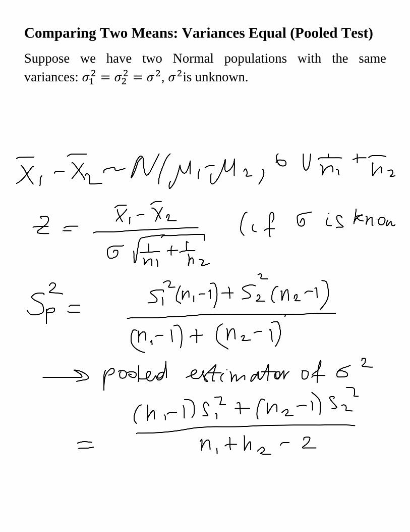
Comparing Two Means: Variances Equal (Pooled Test)

Suppose we have two Normal populations with the same

variances:

, is unknown.

The pooled two-sample t procedures:

Choose an SRS of size from a Normal population with

unknown mean and an independent SRS of size from

another Normal population with unknown mean .

A CI for is given by

√

where is the value for density curve with area

between and .

To test the hypothesis , compute the pooled two-

sample t statistic

√

In terms of a random variable T having the distribution,

the P-value for a test of against

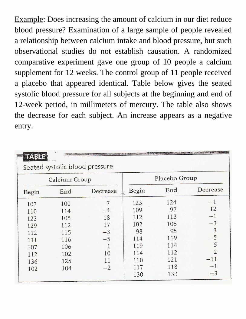
Example: Does increasing the amount of calcium in our diet reduce

blood pressure? Examination of a large sample of people revealed

a relationship between calcium intake and blood pressure, but such

observational studies do not establish causation. A randomized

comparative experiment gave one group of 10 people a calcium

supplement for 12 weeks. The control group of 11 people received

a placebo that appeared identical. Table below gives the seated

systolic blood pressure for all subjects at the beginning and end of

12-week period, in millimeters of mercury. The table also shows

the decrease for each subject. An increase appears as a negative

entry.

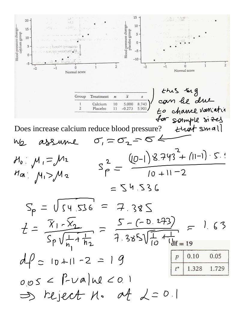
Does increase calcium reduce blood pressure?

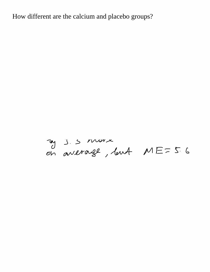
How different are the calcium and placebo groups?

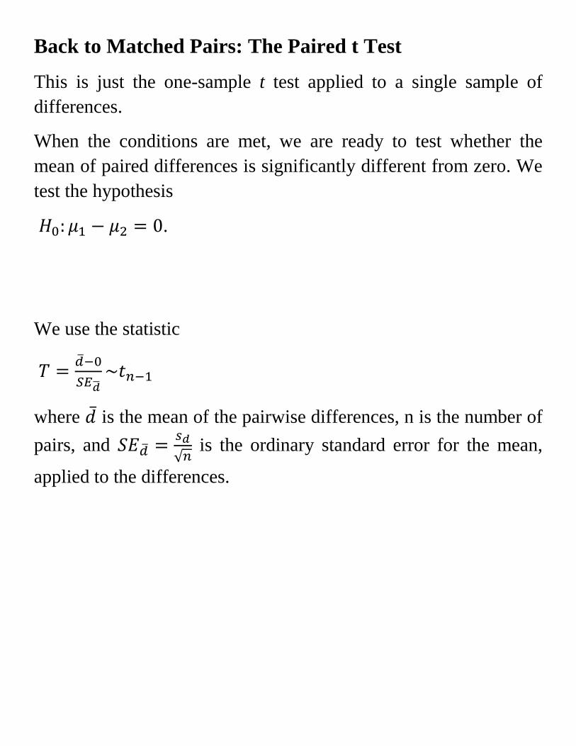
Back to Matched Pairs: The Paired t Test

This is just the one-sample t test applied to a single sample of

differences.

When the conditions are met, we are ready to test whether the

mean of paired differences is significantly different from zero. We

test the hypothesis

.

We use the statistic

where is the mean of the pairwise differences, n is the number of

pairs, and

√ is the ordinary standard error for the mean,

applied to the differences.

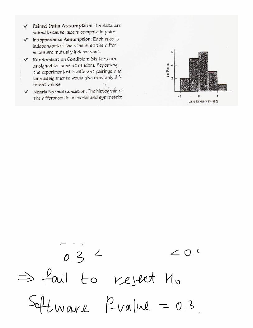
Example: Speed-skating races are run in pairs. Two skaters start at

the same time, one on the inner lane and one on the outer lane.

Halfway through the race they cross over, switching lanes so that

each will skate the same distance in each lane. Even though this

seems fair, at the 2006 Olympics some fans thought there might

have been an advantage to starting on the outside. Here are the data

for women’s 1500-m race:

Was there are a difference in speeds between the inner and outer

speed-skating lanes at the 2006 Winter Olympics?

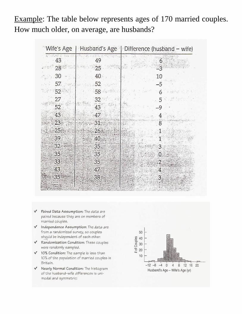
Example: The table below represents ages of 170 married couples.

How much older, on average, are husbands?

, ,

Alternative Nonparametric Methods:

The Wilcoxon Rank Sum Test

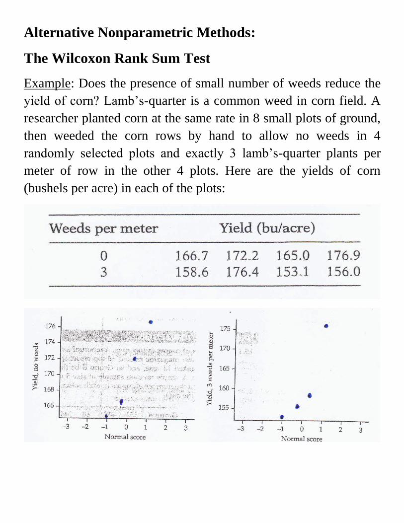
Example: Does the presence of small number of weeds reduce the

yield of corn? Lamb’s-quarter is a common weed in corn field. A

researcher planted corn at the same rate in 8 small plots of ground,

then weeded the corn rows by hand to allow no weeds in 4

randomly selected plots and exactly 3 lamb’s-quarter plants per

meter of row in the other 4 plots. Here are the yields of corn

(bushels per acre) in each of the plots:

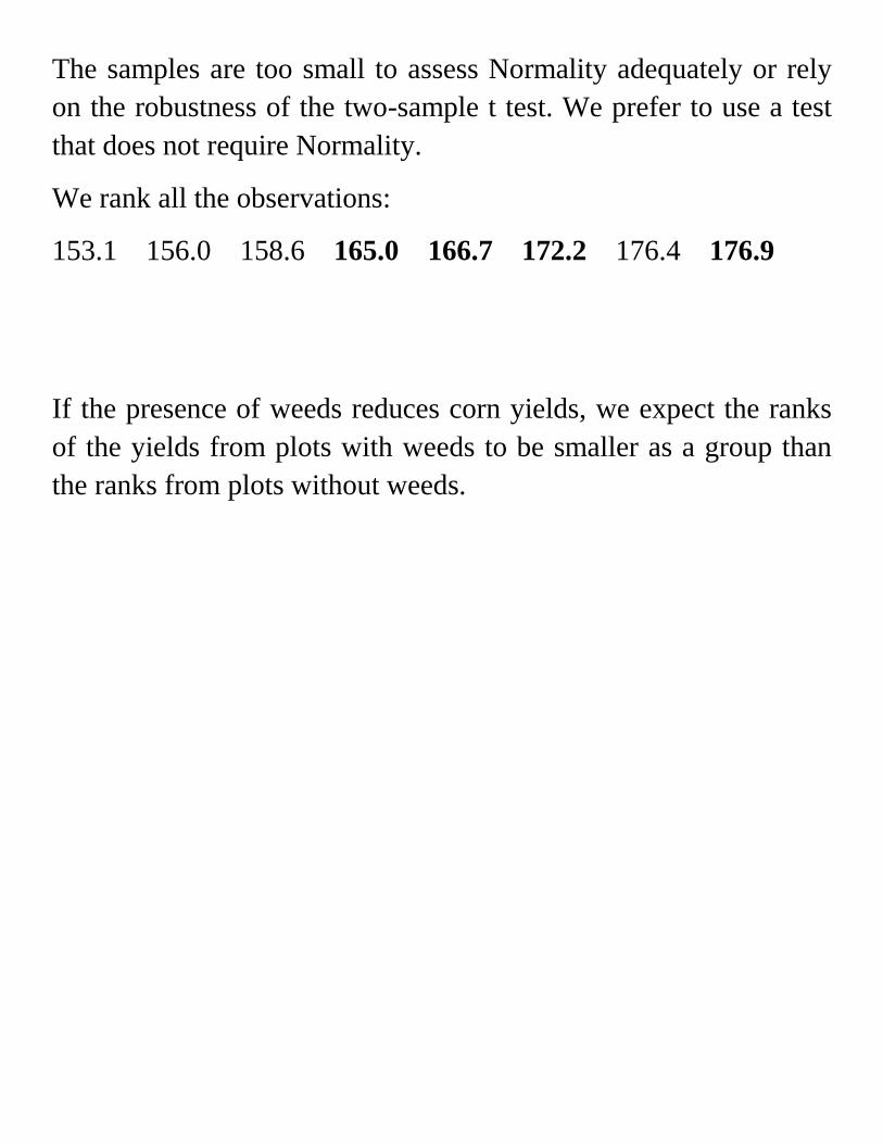
The samples are too small to assess Normality adequately or rely

on the robustness of the two-sample t test. We prefer to use a test

that does not require Normality.

We rank all the observations:

153.1 156.0 158.6 165.0 166.7 172.2 176.4 176.9

If the presence of weeds reduces corn yields, we expect the ranks

of the yields from plots with weeds to be smaller as a group than

the ranks from plots without weeds.

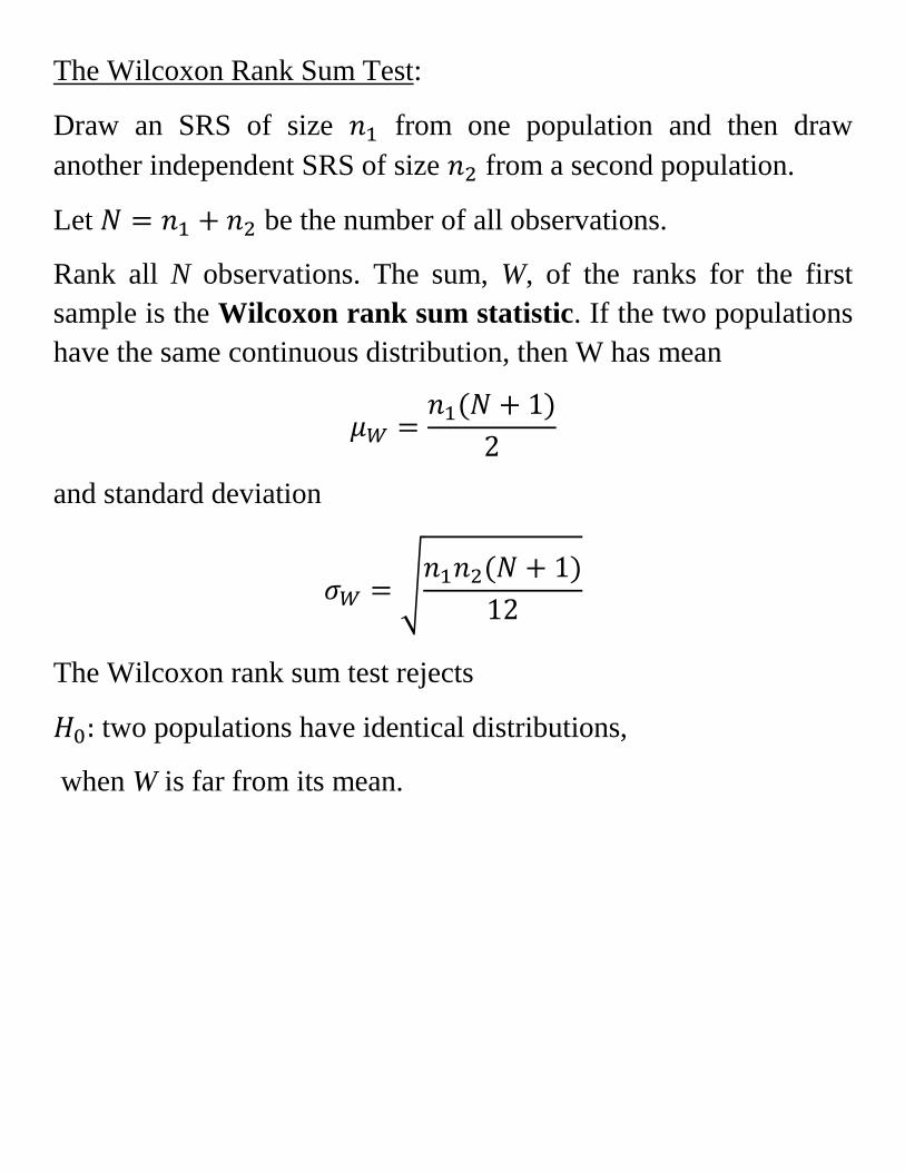
The Wilcoxon Rank Sum Test:

Draw an SRS of size from one population and then draw

another independent SRS of size from a second population.

Let be the number of all observations.

Rank all N observations. The sum, W, of the ranks for the first

sample is the Wilcoxon rank sum statistic. If the two populations

have the same continuous distribution, then W has mean

and standard deviation

√

The Wilcoxon rank sum test rejects

two populations have identical distributions,

when W is far from its mean.

Back to our corn example:

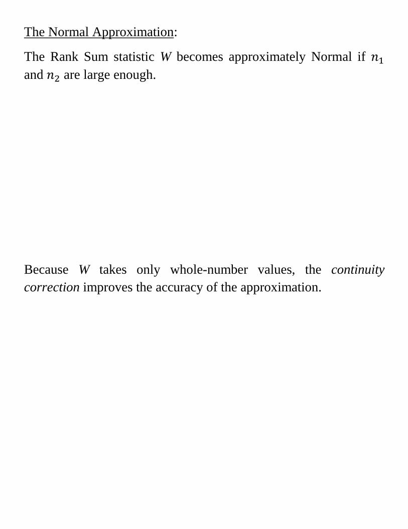
The Normal Approximation:

The Rank Sum statistic W becomes approximately Normal if

and are large enough.

Because W takes only whole-number values, the continuity

correction improves the accuracy of the approximation.