Lecture 7 (D. Geman)

7/29/2019 Lecture 7 (D. Geman)

http://slidepdf.com/reader/full/lecture-7-d-geman 1/67

STATISTICAL LEARNING IN CANCERBIOLOGY: LECTURE 7

Donald Geman, Michael Ochs, Laurent YounesJohns Hopkins Unversity

ENS-Cachan

February 27, 2013



LECTURE SERIES

Lecture 1: Introduction (DG)

Lecture 2: Cancer Biology (MO)

Lecture 3: Cell Signaling Inference (MO)

Lecture 4: Genetic Variation (DG)

Lecture 5: Massive Testing (LY)

Lecture 6: Biomarker Discovery (LY)

Lecture 7: Phenotype Prediction (DG) Lecture 8: Embedding Mechanism (DG)

2 / 64



OUTLINE

Biology and Statistical Learning

Predicting from Comparisons Pathway De-regulation

Breast Cancer Prognosis

Metastatic Cancer

3 / 64



RECAP

Statistical methods for analyzing cancer data permeate the

literature.

Prominent examples examined in previous lectures include Modeling the accumulation of driver mutations during

tumorigenesis; Identifying perturbed signaling in tumor cells; Discovering risk-bearing DNA sequence variation; and Finding differentially expressed genes and gene products.

The final two lectures are about learning classifiers that candistinguish between cellular phenotypes from mRNA

transcript levels collected from cells in assayed tissue.

4 / 64



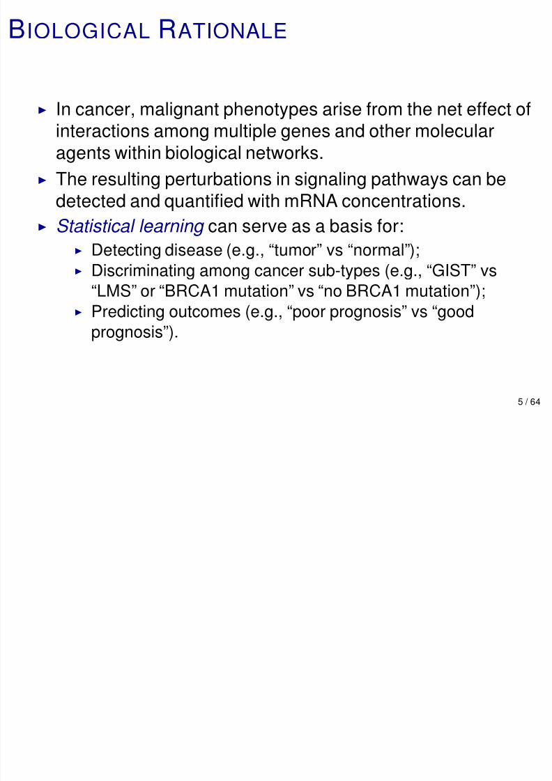
BIOLOGICAL RATIONALE

In cancer, malignant phenotypes arise from the net effect of

interactions among multiple genes and other molecular

agents within biological networks.

The resulting perturbations in signaling pathways can be

detected and quantified with mRNA concentrations.

Statistical learning can serve as a basis for: Detecting disease (e.g., “tumor” vs “normal”); Discriminating among cancer sub-types (e.g., “GIST” vs

“LMS” or “BRCA1 mutation” vs “no BRCA1 mutation”); Predicting outcomes (e.g., “poor prognosis” vs “good

prognosis”).

5 / 64



STATISTICAL LEARNING (I)

X : High-throughput genomic data.

The traditional approach – experimental and

molecule-by-molecule – is not feasible at this scale. A principled approach is required to extract knowledge from

X.

Statistical learning has emerged as a core methodology for

the analysis of X.

6 / 64



STATISTICAL LEARNING (II)

Training set: L = (x(1), y (1)), . . . , (x(n ), y (n )). x(i ) ∈ Rd : mRNA expression profile for sample i ; y (i ) ∈ 1, 2, ..., K : cellular phenotype of sample i .

Standard Goals: Learn a predictor f : Rd −→ 1, ..., K or

class-conditional model p (x|k ) from L.

Less Standard: Develop statistical metrics and models for

regulation and mechanism.

7 / 64



BARRIERS (I)

Applications to biomedicine, specifically the implications for

clinical practice, are widely acknowledged to remain limited.

One major barrier is the study-to-study diversity in reported

prediction accuracies and “signatures” (lists of

discriminating genes).

Some of this variation can be attributed to the over-fitting

that results from the infamous “small n, large d” dilemma.

Typically, the number of samples (chips, profiles, patients)

per class is n = 10 − 1000 whereas the number of features

(exons, transcripts, genes) is d = 1000− 50, 000.

8 / 64



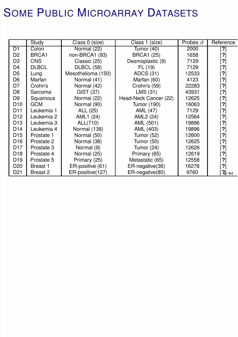
SOME PUBLIC MICROARRAY DATASETS

Study Class 0 (size) Class 1 (size) Probes d ReferenceD1 Colon Normal (22) Tumor (40) 2000 [?]D2 BRCA1 non-BRCA1 (93) BRCA1 (25) 1658 [?]D3 CNS Classic (25) Desmoplastic (9) 7129 [?]D4 DLBCL DLBCL (58) FL (19) 7129 [?]D5 Lung Mesothelioma (150) ADCS (31) 12533 [?]D6 Marfan Normal (41) Marfan (60) 4123 [?]

D7 Crohn’s Normal (42) Crohn’s (59) 22283 [?]D8 Sarcoma GIST (37) LMS (31) 43931 [?]D9 Squamous Normal (22) Head-Neck Cancer (22) 12625 [?]D10 GCM Normal (90) Tumor (190) 16063 [?]D11 Leukemia 1 ALL (25) AML (47) 7129 [?]D12 Leukemia 2 AML1 (24) AML2 (24) 12564 [?]

D13 Leukemia 3 ALL(710) AML (501) 19896 [?]D14 Leukemia 4 Normal (138) AML (403) 19896 [?]D15 Prostate 1 Normal (50) Tumor (52) 12600 [?]D16 Prostate 2 Normal (38) Tumor (50) 12625 [?]D17 Prostate 3 Normal (9) Tumor (24) 12626 [?]D18 Prostate 4 Normal (25) Primary (65) 12619 [?]D19 Prostate 5 Primary (25) Metastatic (65) 12558 [?]

D20 Breast 1 ER-positive (61) ER-negative(36) 16278 [?]D21 Breast 2 ER-positive(127) ER-negative(80) 9760 [?]9 / 64



BARRIERS (II)

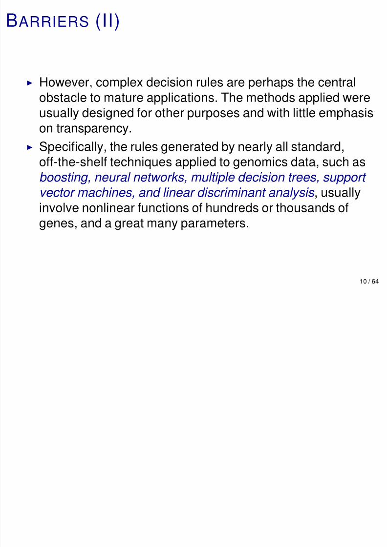
However, complex decision rules are perhaps the central

obstacle to mature applications. The methods applied were

usually designed for other purposes and with little emphasis

on transparency.

Specifically, the rules generated by nearly all standard,

off-the-shelf techniques applied to genomics data, such as

boosting, neural networks, multiple decision trees, support vector machines, and linear discriminant analysis , usually

involve nonlinear functions of hundreds or thousands ofgenes, and a great many parameters.

10 / 64



BARRIERS (IV)

Consequently, standard decision rules are too complex to characterize biologically.

Moreover, what is notably missing is a solid link with potential mechanism, which seem to be a necessary

condition for “translational medicine”, i.e., drug development

and clinical decision-making.

12 / 64



ACCURACY AND CONTEXT

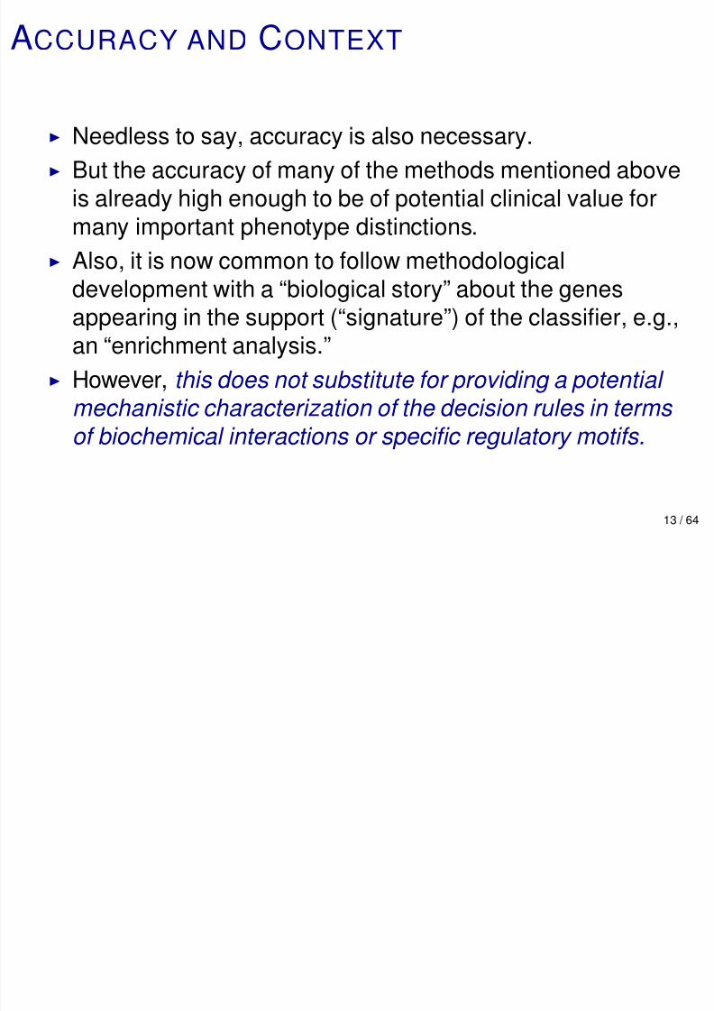
Needless to say, accuracy is also necessary.

But the accuracy of many of the methods mentioned above

is already high enough to be of potential clinical value for

many important phenotype distinctions.

Also, it is now common to follow methodologicaldevelopment with a “biological story” about the genes

appearing in the support (“signature”) of the classifier, e.g.,

an “enrichment analysis.”

However, this does not substitute for providing a potential mechanistic characterization of the decision rules in terms

of biochemical interactions or specific regulatory motifs.

13 / 64



PROPOSED FRAMEWORK

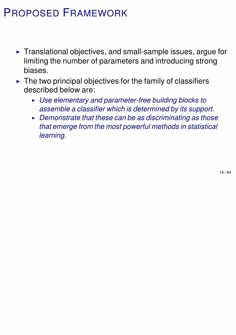
Translational objectives, and small-sample issues, argue for

limiting the number of parameters and introducing strong

biases.

The two principal objectives for the family of classifiersdescribed below are: Use elementary and parameter-free building blocks to

assemble a classifier which is determined by its support. Demonstrate that these can be as discriminating as those

that emerge from the most powerful methods in statistical learning.

14 / 64



EXPRESSION ORDERING

The building blocks we choose are two-gene comparisons,

regarded as “biological switches” related to regulatory

“motifs” or other properties of transcriptional networks.

The decision rules are then determined by expression orderings .

However, explicitly connecting statistical classification and molecular mechanism for cancer is a major, largely open,

challenge.

A more modest goal is to propose a potential statistical

framework.

15 / 64



OUTLINE


Predicting from Comparisons

Pathway De-regulation


Metastatic Cancer

16 / 64



STRATEGY

Use (within sample) ranks to enhance robustness.

Adapt models to sample size.

Introduce bias to control variance.

Bias towards potential mechanism.

Hypothesis-driven learning?

17 / 64



NOTATION (I)

G : list of d genes.

X = (X 1, ..., X d ): expression profile.

Y ∈ 1, 2, ..., K : classes or phenotypes.

Data: d × n matrix of mRNA counts.

May restrict G to a network m with d m genes.

18 / 64



NOTATION (II)

Order the expression values: x π1≤ · · · ≤ x πd

.

Let r i be the rank of gene i in the ordering.

Then r = (r 1, ..., r d ) ∈ Ωd , the set of permutations of1, ..., d , and r = π−1.

Thus, x i < x j for two genes i , j if and only if r i < r j .

Replace x ∈ Rd by r ∈ Ωd .

Define binary variables z ij = δ (r i < r j ).

19 / 64



NOTATION (III)

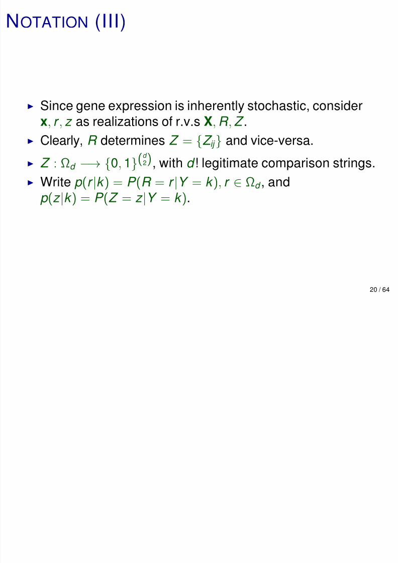
Since gene expression is inherently stochastic, consider

x, r , z as realizations of r.v.s X, R , Z .

Clearly, R determines Z = Z ij and vice-versa. Z : Ωd −→ 0, 1(d

2), with d ! legitimate comparison strings.

Write p (r |k ) = P (R = r |Y = k ), r ∈ Ωd , and

p (z |k ) = P (Z = z |Y = k ).

20 / 64

E O Z C B D



EVEN ONE Z ij CAN BE DISCRIMINATING

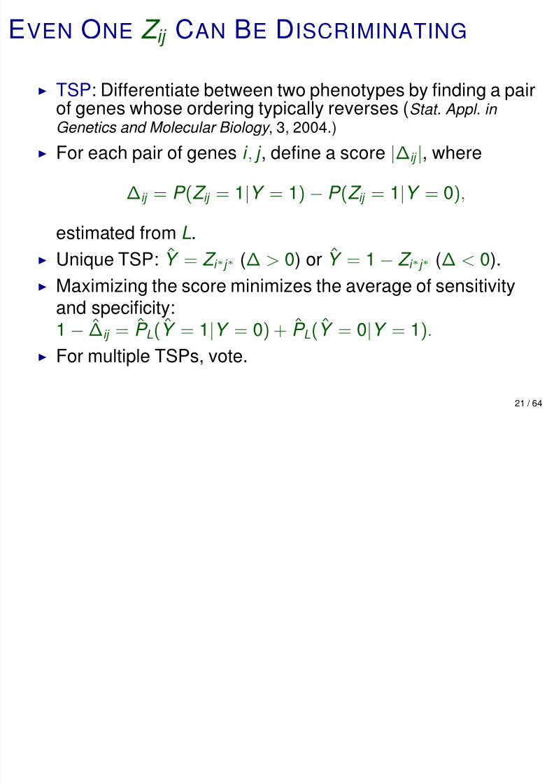
TSP: Differentiate between two phenotypes by finding a pairof genes whose ordering typically reverses (Stat. Appl. in Genetics and Molecular Biology , 3, 2004.)

For each pair of genes i , j , define a score |∆ij |, where

∆ij = P (Z ij = 1|Y = 1) − P (Z ij = 1|Y = 0),

estimated from L.

Unique TSP: Y = Z i ∗ j ∗ (∆ > 0) or Y = 1− Z i ∗ j ∗ (∆ < 0).

Maximizing the score minimizes the average of sensitivityand specificity:

1 − ∆ij = P L(Y = 1|Y = 0) + P L(Y = 0|Y = 1).

For multiple TSPs, vote.

21 / 64

A “N F L ” E B



A “NO FREE LUNCH” ERROR BOUND

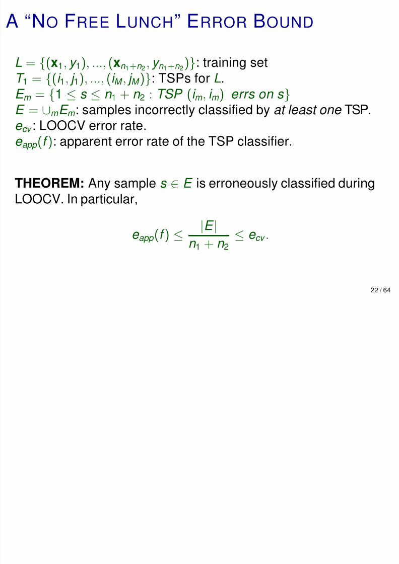
L = (x1, y 1), ..., (xn 1+n 2 , y n 1+n 2 ): training set

T 1 = (i 1, j 1), ..., (i M , j M ): TSPs for L.

E m = 1 ≤ s ≤ n 1 + n 2 : TSP (i m , i m ) errs on s E = ∪m E m : samples incorrectly classified by at least one TSP.

e cv : LOOCV error rate.

e app (f ): apparent error rate of the TSP classifier.

THEOREM: Any sample s ∈ E is erroneously classified during

LOOCV. In particular,

e app (f ) ≤|E |

n 1 + n 2≤ e cv .

22 / 64

K T S P



K TOP SCORING PAIRS

Base prediction on the k highest scoring pairs:

Θ∗k = (i 1, j 1), . . . , (i k , j k ).

More generally, the natural discriminant is

g k (X; Θk ) =

(i , j )∈Θk

δ X i < X j

The k-TSP classifier is majority voting:

f (X) = δ g k (X : Θk ) >

k

2

Varying the threshold allows for trading off sensitivity and

specificity.

23 / 64

C OOS G



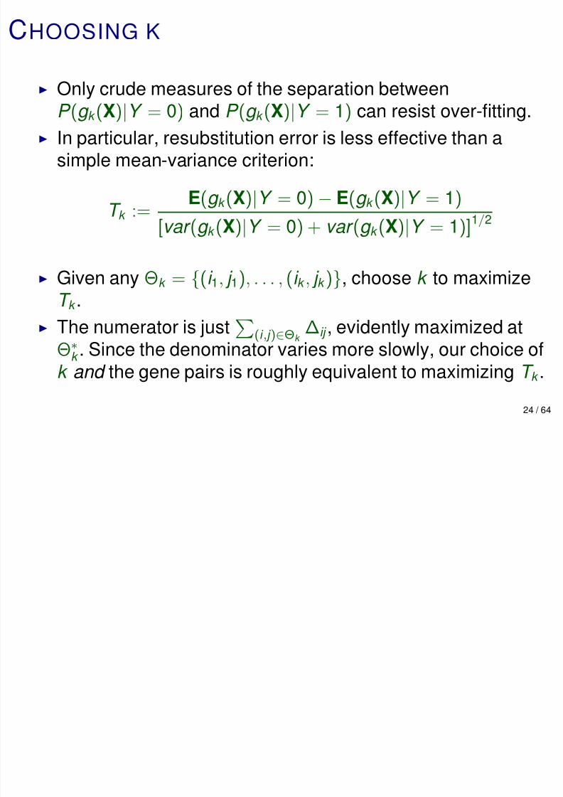
CHOOSING K

Only crude measures of the separation between

P (g k (X)|Y = 0) and P (g k (X)|Y = 1) can resist over-fitting.

In particular, resubstitution error is less effective than a

simple mean-variance criterion:

T k := E(g k (X)|Y = 0) − E(g k (X)|Y = 1)[var (g k (X)|Y = 0) + var (g k (X)|Y = 1)]1/2

Given any Θk = (i 1, j 1), . . . , (i k , j k ), choose k to maximize

T k . The numerator is just

(i , j )∈Θk

∆ij , evidently maximized at

Θ∗

k . Since the denominator varies more slowly, our choice of

k and the gene pairs is roughly equivalent to maximizing T k .

24 / 64

FURTHER HOMEGROWN DEVELOPMENTS



FURTHER HOMEGROWN DEVELOPMENTS

Comparisons with discriminative methods (SVM, PAM,

k-NN, RF, naive Bayes) on “standard” cancer datasets:

“Simple decision rules for classifying human cancers from gene

expression profiles,” Bioinformatics , 21, 3896-3904, 2005.

Specialized to prostate cancer: “Robust prostate cancer

marker genes discovered from direct integration of inter-study

microarray data,” 21, 3905-3911, Bioinformatics , 2005.

25 / 64

EXTERNAL VALIDATION



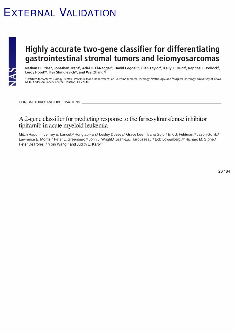
EXTERNAL VALIDATION

Highly accurate two-gene classifier for differentiatinggastrointestinal stromal tumors and leiomyosarcomasNathan D. Price*, Jonathan Trent†, Adel K. El-Naggar‡, David Cogdell‡, Ellen Taylor‡, Kelly K. Hunt§, Raphael E. Pollock§,Leroy Hood*¶, Ilya Shmulevich*, and Wei Zhang‡ʈ

*Institute for Systems Biology, Seattle, WA 98103; and Departments of †Sarcoma Medical Oncology, ‡Pathology, and §Surgical Oncology, University of TexasM. D. Anderson Cancer Center, Houston, TX 77030

CLINICAL TRIALS AND OBSERVATIONS

A2-gene classifier for predicting response to the farnesyltransferase inhibitor

tipifarnib in acute myeloid leukemiaMitch Raponi,1 Jeffrey E. Lancet,2 Hongtao Fan,3 Lesley Dossey,1 Grace Lee,1 Ivana Gojo,4 Eric J. Feldman,5 Jason Gotlib,6

Lawrence E. Morris,7 Peter L. Greenberg,6 John J. Wright,8 Jean-Luc Harousseau,9 Bob Lowenberg,10 Richard M. Stone,11

Peter De Porre,12 Yixin Wang,1 and Judith E. Karp13

26 / 64

EXTERNAL VALIDATION (CONT)



EXTERNAL VALIDATION (CONT)

ORIGINAL ARTICLE

Usefulness of the top-scoring pairs of genes for predictionof prostate cancer progression

H Zhao, CJ Logothetis and IP GorlovDepartment of Genitourinary Medical Oncology, The University of Texas MD, Anderson Cancer Center, Houston, TX, USA

Prostate Cancer and Prostatic Diseases (2010), 1– 8& 2010 Nature Publishing Group All rights reserved 1365-7852/10 $32.00

www.nature.com/pcan

An interferon-related gene signature for DNA damageresistance is a predictive marker for chemotherapyand radiation for breast cancerRalph R. Weichselbauma,b, Hemant Ishwaranc, Taewon Yoona,b, Dimitry S. A. Nuytend,e, Samuel W. Bakera,b,Nikolai Khodareva, Andy W. Sua,b, Arif Y. Shaikha,b, Paul Roachf, Bas Kreiked,e, Bernard Roizmang, Jonas Berghh,Yudi Pawitani, Marc J. van de Vijverd, and Andy J. Minna,b,1

27 / 64

TOP SCORING MEDIANS (TSM)



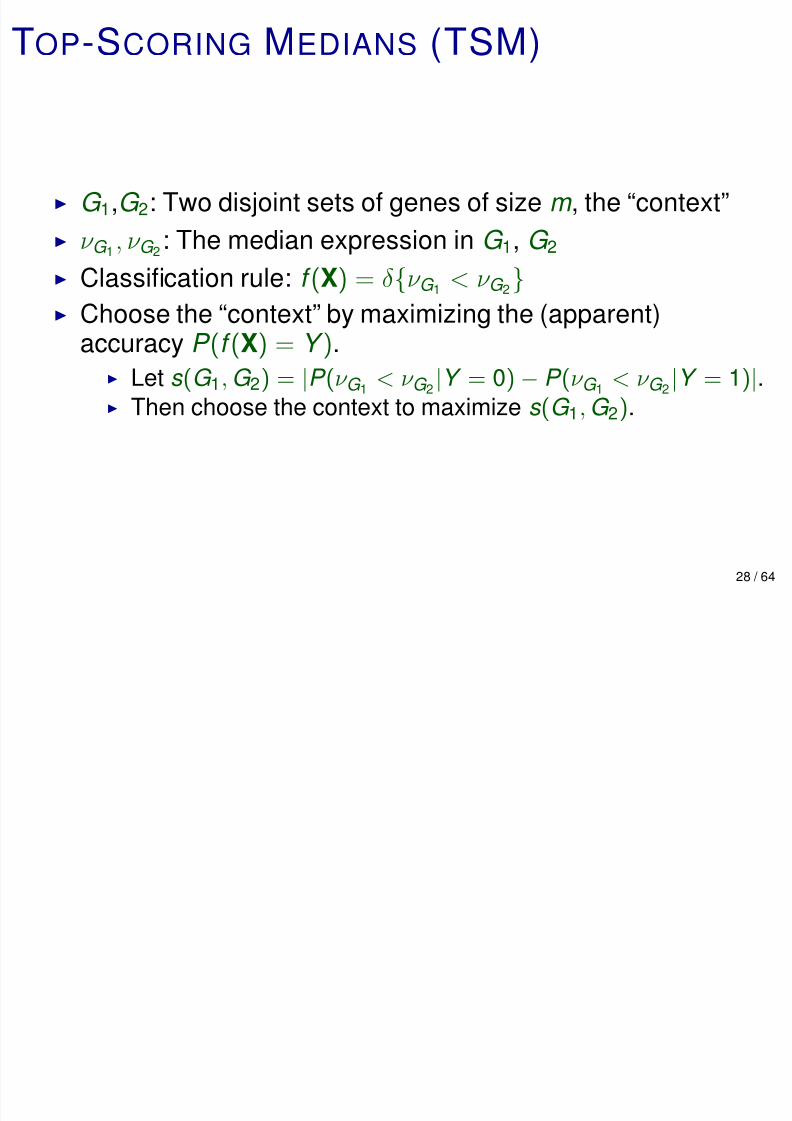
TOP-SCORING MEDIANS (TSM)

G 1,G 2: Two disjoint sets of genes of size m , the “context”

ν G 1 , ν G 2 : The median expression in G 1, G 2

Classification rule: f (X) = δ ν G 1 < ν G 2 Choose the “context” by maximizing the (apparent)

accuracy P (f (X) = Y ). Let s (G 1, G 2) = |P (ν G 1 < ν G 2 |Y = 0)− P (ν G 1 < ν G 2 |Y = 1)|. Then choose the context to maximize s (G 1, G 2).

28 / 64

FINDING THE CONTEXT (I)



FINDING THE CONTEXT (I)

Exact optimization (for m > 1) is computationally impossibleand would lead to massive overfitting anyway.

Let ν G 1 = R π1, ν G 2 = R π2

(ranks are computed in G 1 ∪G 2).

Suppose:

(i) X i < X j ⊥ π1 = i , π2 = j |Y for each i ∈ G 1, j ∈ G 2;(ii) (π1, π2) is uniformly distributed given Y .

Then

P (ν G 1 < ν G 2|Y ) =1

m 2 i ∈G 1, j ∈G 2

P (X i < X j |Y ).

29 / 64

FINDING THE CONTEXT (II)



FINDING THE CONTEXT (II)

Both assumptions are true in practice. Consequently,

s (G 1, G 2) ∝

i ∈G 1, j ∈G 2 ∆ij .

Finally,

( G 1, G 2) = arg maxG 1,G 2 i ∈G 1, j ∈G 2

∆ij

This search is feasible either (i) exactly, but with gene

filtering, for m ≈ 5; or (ii) greedily, adding one gene at a

time, without gene filtering.

30 / 64

CLASSIFICATION RESULTS



CLASSIFICATION RESULTS

31 / 64

OUTLINE



OUTLINE





Metastatic Cancer

32 / 64

PERTURBED NETWORKS



PERTURBED NETWORKS

Diseased cells arise from aberrant activity in cellular

signaling, and pathways are the fundamental scale of many

cancer processes.

These aberrations cannot be identified from phenotypic

information typically measured in the clinic.

Moreover, they are the net effect of interactions among

multiple molecular agents.

Generally, network analyses do not account for

combinatorial (multi-way) interactions among genes or geneproducts, and do not quantify de-regulation.

33 / 64

BABY ILLUSTRATION



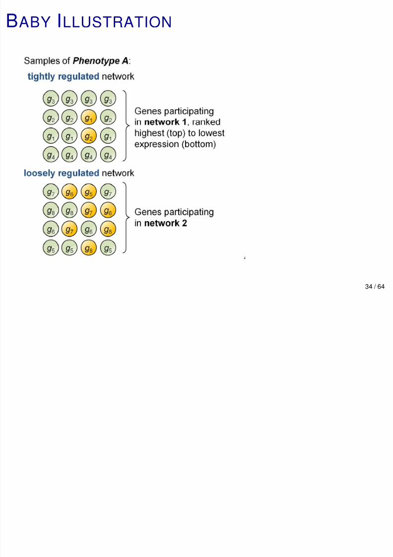
BABY ILLUSTRATION

34 / 64

SWAP DISTANCE



SWAP DISTANCE

A distance between permutations π and π of 1, . . . , d .

D (π, π

): the minimum number of adjacent swaps needed totransform π into π.

Example: D ((3, 1, 2, 4), (1, 2, 3, 4)) = 2.

35 / 64

PATHWAY VARIABLES



PATHWAY VARIABLES

Consider a network m with d m genes.

Let π = (π1, . . . , πd m ) be the order statistics for

x = (x 1, . . . , x d m ): x π1

< x π2

< · · · < x πd m

.

Let D (x, x) be the swap distance between π(x) and π(x).

Then D (x, x) is also the normalized Hamming distance

between z (x ) and z (x ), the corresponding comparison

strings.

36 / 64

ORDER INDEX



ORDER INDEX

Fix a phenotype k and let X and X

be i.i.d. expressionprofiles under p (x|k ).

Define the Order Index : µ(k ,m ) = 1−

d m

2

−1E[D (X, X)].

Then it is easy to show that

µ(k ,m ) = 1−d m

2

−1 i , j ∈G m

2P (Z ij = 1|k )P (Z ij = 0|k ).

.5 ≤ µ ≤ 1, but generally µ .5 since there are many genepairs expressed on different scales.

µ(k ,m ) 1: A highly disorganized system.

37 / 64

EXAMPLES



EXAMPLES

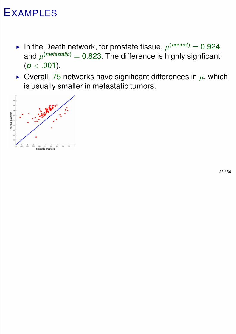
In the Death network, for prostate tissue, µ(normal ) = 0.924and µ(metastatic ) = 0.823. The difference is highly signficant

(p < .001).

Overall, 75 networks have significant differences in µ, which

is usually smaller in metastatic tumors.

38 / 64

DE-REGULATION IN DISEASE



GU O S S

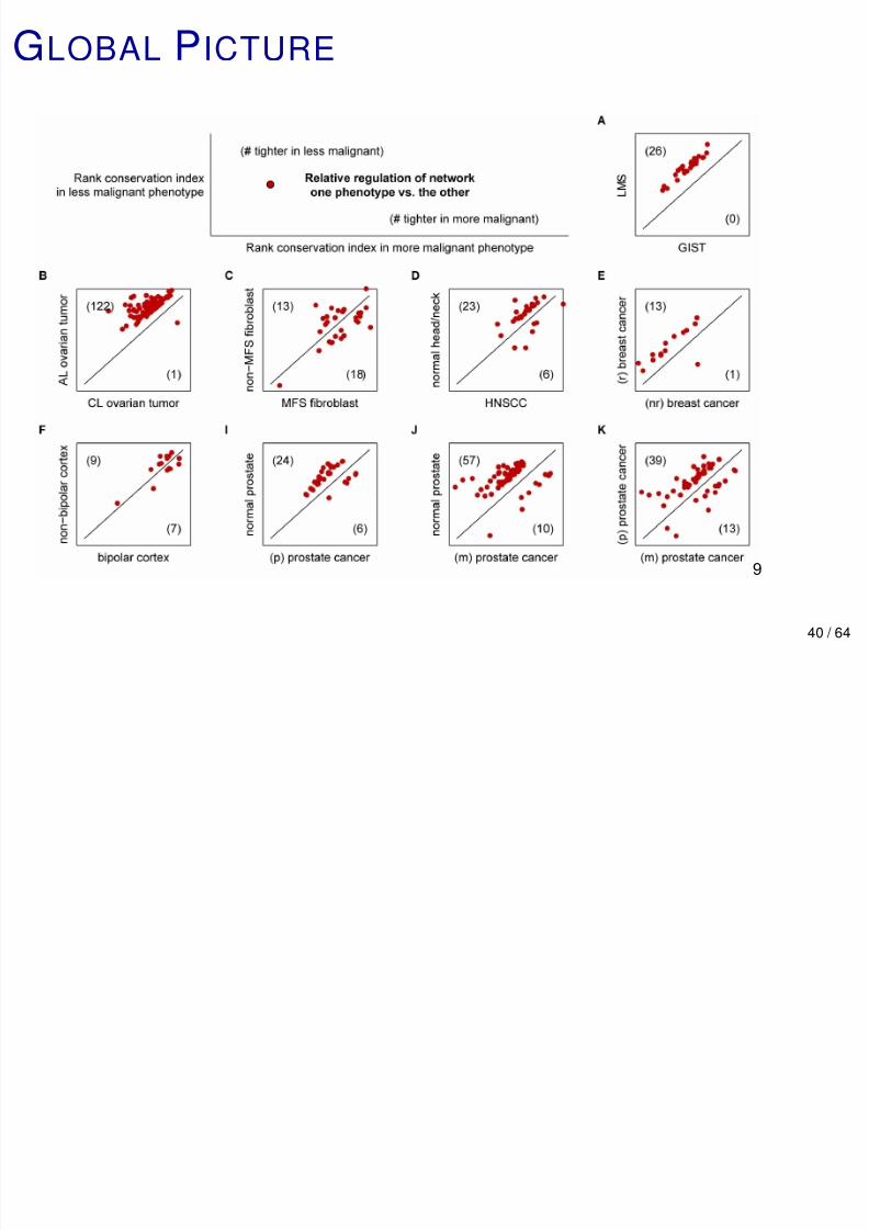
A general trend emerges: when pairs of phenotypes

represent gradations of disease, the order index is usually smaller in the more malignant one when there is a

significant difference.

In the following plots, each point represents a pair

(µ(A,m ), µ(B ,m )) for a network m , where A is more malignant

than B.

39 / 64

GLOBAL PICTURE



9

40 / 64

DISTANCE-BASED CLASSIFICATION



Fix a context G (set of genes).

Let D G be the swap distance restricted to G .

Classify by nearest-neighbor in L.

Choose G so that the distance D G (X, X’) betweenindependent samples is

Large if X, X are from different classes; Small if from the same class.

This can be done in a similar fashion to kTSP and TSM.

41 / 64

OUTLINE







Metastatic Cancer

42 / 64

BREAST CANCER PROGNOSIS



Objective: separate BC microarray samples into “good” vs“poor” prognosis determined by recurrence within five years.

Mammaprint Signature: List of 70 genes and corresponding

(correlation-based) decision rule.

One of three “signatures” approved by the FDA for clinicaluse.

Learned from a training set L with n = 162 samples (46

recurrent and 116 non-recurrent).

Achieves 89% sensitivity and 41% specificity on the Buysetest set of n = 302 samples (46 recurrent and 256

non-recurrent).

43 / 64

MAXIMUM ENTROPY MODELS ON



PERMUTATIONS

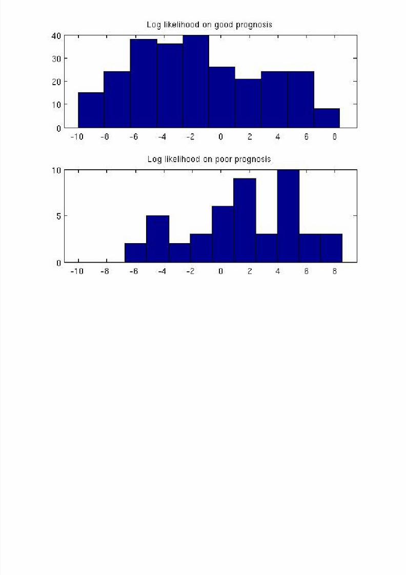
Fix ten genes (e.g., the five top-scoring pairs).

Let x be the expression profile and r ∈ Ω10 the rank vector.

Construct two distributions p (r |good ) and p (r |poor ) bymaximizing entropy subject to fixing all

102

= 45 pairwise

comparison probabilities.

Use “Iterative Projection” to learn the parameters.

With d = 10, everything can be computed, includingnormalizing constants and entropies.

44 / 64

MORE FORMALLY



Let q be a prob. dist. on Ω10, and let p L be the empirical

distribution on L.

For k ∈ poor , good :

p (r |k ) = argq max H (q )

s .t . ∀i < j : q (r : r i < r j ) = p L(r : r i < r j |k )

45 / 64



LIKELIHOOD RATIO TEST



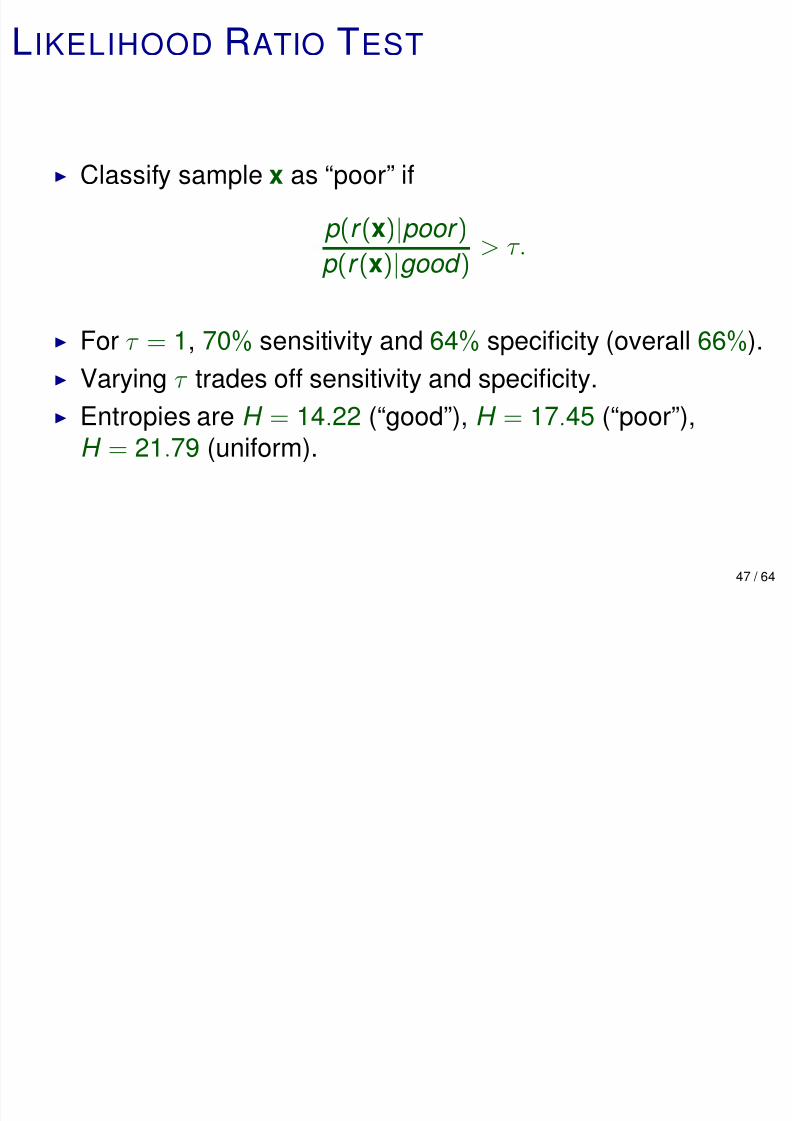
Classify sample x as “poor” if

p (r (x)|poor )

p (r (x)|good )> τ.

For τ = 1, 70% sensitivity and 64% specificity (overall 66%).

Varying τ trades off sensitivity and specificity.

Entropies are H = 14.22 (“good”), H = 17.45 (“poor”),H = 21.79 (uniform).

47 / 64

OUTLINE







Metastatic Cancer

48 / 64

METASTATIC CANCER



Cancer is an acquired genetic disorder due to the

accumulation over time of DNA alterations that lead to

uncontrolled cell growth and proliferation.

Ninety percent of deaths result from metastasis, meaning

that cancer cells break away and migrate to distant organs.

By lodging in other organs they replace normal cells until

the organ no longer functions.

49 / 64

TUMOR SITE OF ORIGIN



In approximately 4% of cancers, a metastatic tumor is found

of unknown primary origin (Hillen, 2000).

However, the appropriate treatment depends on the tissue

of origin.

The GEO or Gene Expression Omnibus (Barrett et al.,

2006) contains 16,715 tumor samples from 20 sites of

origin for the most popular platform.

Objective: Build a classifier for distinguishing among the

20 sites of origin and validate it with cross-study errorestimation.

50 / 64

GENERIC PROBLEM: BATCH EFFECTS



Systematic variation across samples is highly correlated

with date, lab, etc.

Especially problematic when batch “labels” are confounded

with class label.

Affects not only the patterns of expression of individual

genes, but in fact the entire dependency structure, including

correlations.

51 / 64

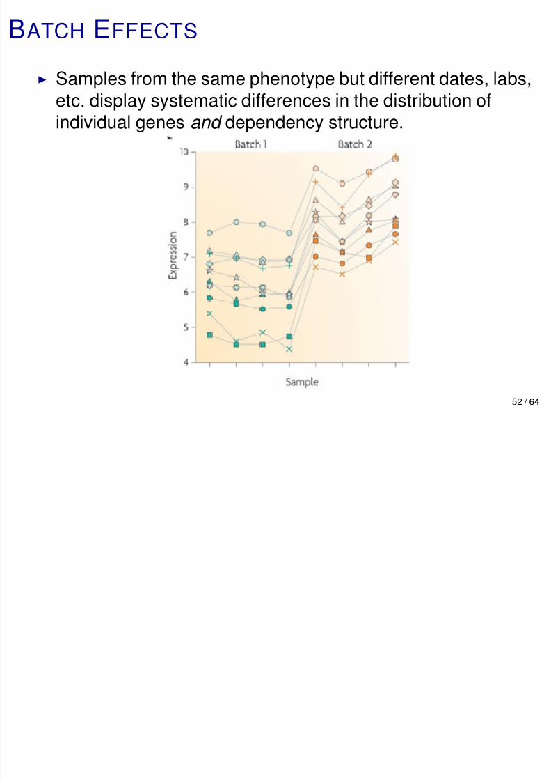
BATCH EFFECTS



Samples from the same phenotype but different dates, labs,

etc. display systematic differences in the distribution ofindividual genes and dependency structure.

52 / 64

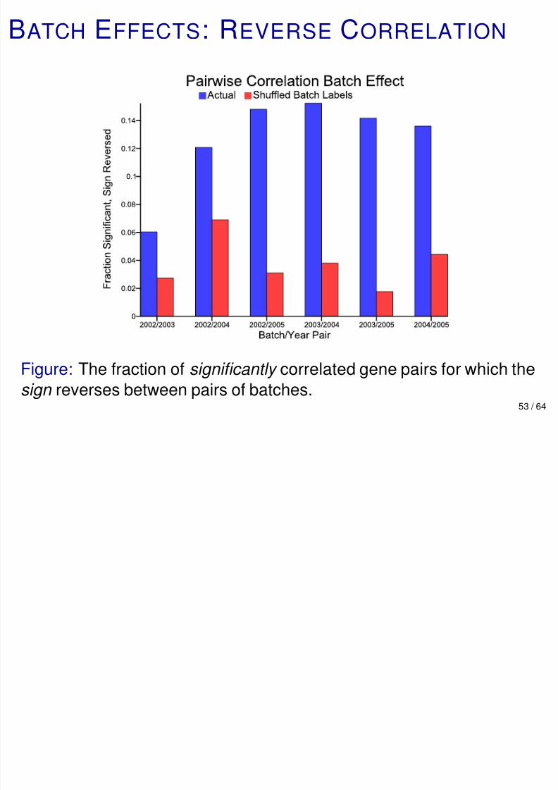
BATCH EFFECTS: REVERSE CORRELATION



Figure: The fraction of significantly correlated gene pairs for which the

sign reverses between pairs of batches.53 / 64

STUDY EFFECTS



Within class, but across studies, there are differences dueto age, location, etc., as well as platform and mRNA

storage/extraction methods.

Combined with batch effects, samples from different studies

are not even approximately identically distributed. Must take this into account in estimating generalization

error.

The consequence of confounding, batch and study effects

make cross-study validation , as opposed to oridinarycross-validation , imperative.

54 / 64

UNBIASED VALIDATION: ACCURACY



Overall accuracy is a poor measure of utility with major

class imbalance in training.

Instead use Mean Class Conditional Accuracy (MCCA). Generalizes the average of sensitivity and specificity to

multiclass.

Take the average of P (F (X ) = y |Y = y ) for y = 1, ..., L.

55 / 64

METHODS OF ESTIMATING ACCURACY



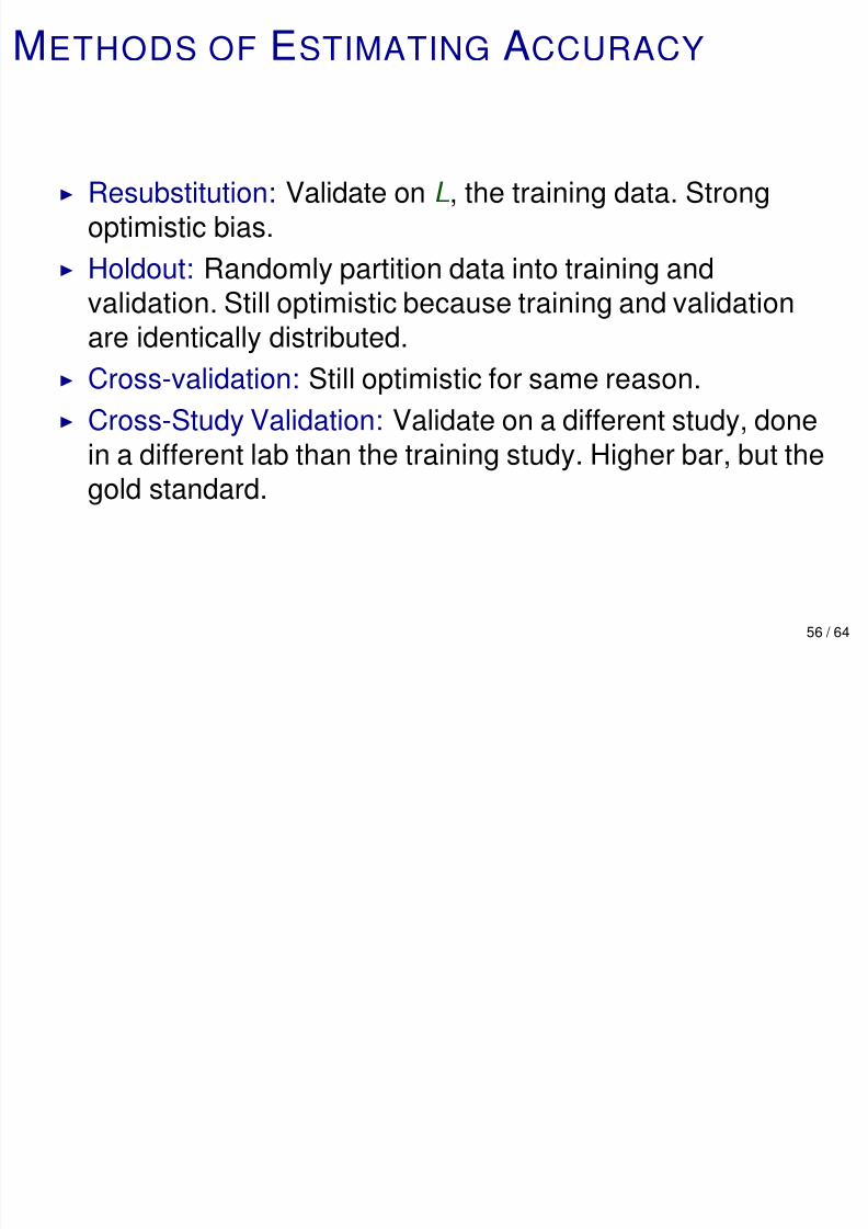
Resubstitution: Validate on L, the training data. Strong

optimistic bias.

Holdout: Randomly partition data into training and

validation. Still optimistic because training and validation

are identically distributed.

Cross-validation: Still optimistic for same reason.

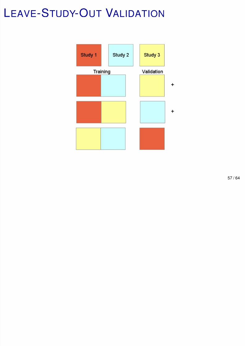
Cross-Study Validation: Validate on a different study, done

in a different lab than the training study. Higher bar, but the

gold standard.

56 / 64

LEAVE-STUDY-OUT VALIDATION



57 / 64

DECISION TREES OF COMPARISONS



Goal: Generalize kTSP and related algorithms to multiclass

problems.

Build decision trees with comparison questions: ”Is gene i more highly expressed than gene j?”

With the site of origin data, can build trees with depth up to

fifteen queries.

58 / 64

TREE OF COMPARISONS



59 / 64

TSP TREES: RESULTS



One decision tree: 91.4% accuracy, 75.4% MCCA. Random Forest with 10 trees and 10k gene pairs chosen at

random for each tree: 95.8% accuracy, 84.2% MCCA

Three trees with no common genes: 94.4% accuracy,

79.9% MCCA Lack of independence problematic for ensembles, even if

disjoint.

Tree 1 Wrong Tree 1 CorrectTree 2 Wrong 741 868Tree 2 Correct 690 14416

60 / 64

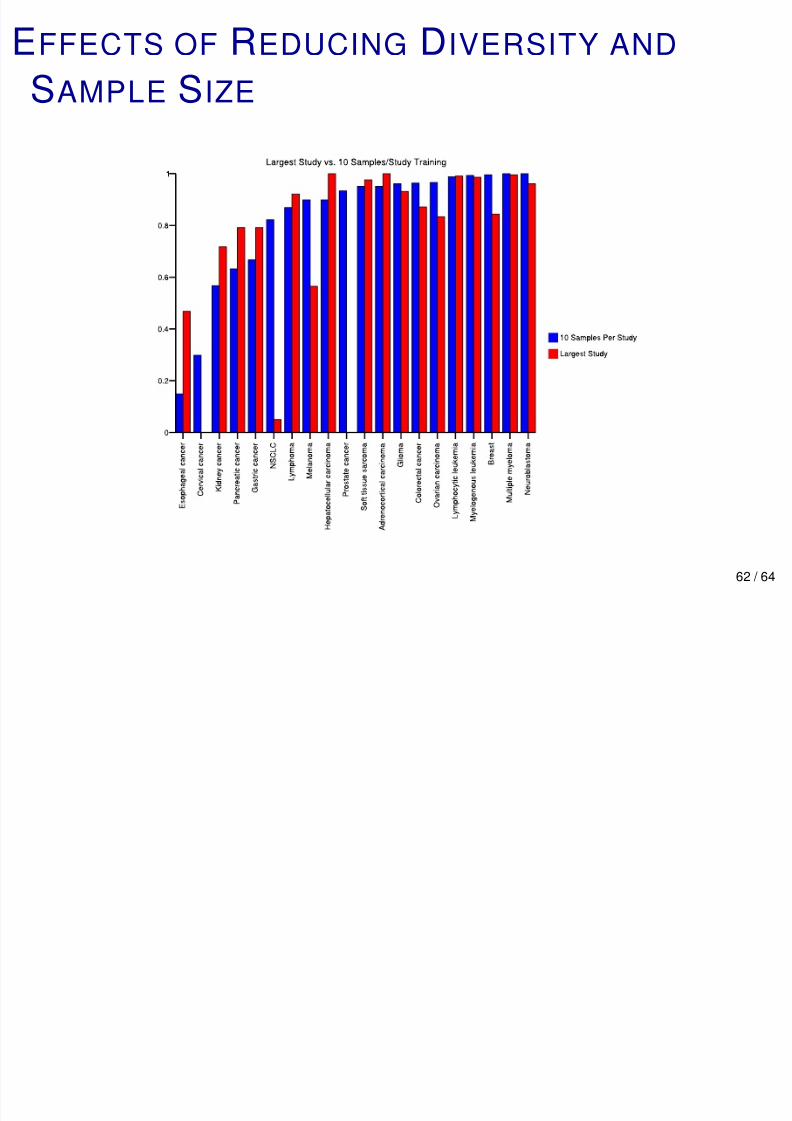
REDUCING DIVERSITY AND SAMPLE SIZE



Reducing Diversity: Train on largest study for each site.

Test on the rest. Accuracy = 85.8%, MCCA = 74.0%.

Reducing n: Keep only 10 samples per study-site of origin

pair. Notice that n is smaller for every site of origin.

61 / 64

EFFECTS OF REDUCING DIVERSITY AND

SAMPLE SIZE



SAMPLE SIZE

62 / 64

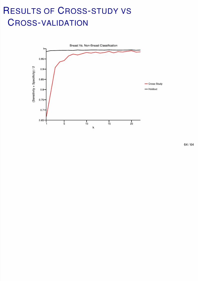
BREAST VS NON-BREAST: CROSS-STUDY VS

HOLDOUT



HOLDOUT

An experiment to compare the performance of cross-study

and (randomized) CV.

Breast vs all 19 other sites.

For non-breast samples, half for training and testing. Randomly order the breast tumor studies. Let n k be the

sample size study k .

Cross-study: Train on studies 1 thru k and validate on study

k + 1. Cross-validation: Randomly choose n k +1 breast samples

from studies 1, ..., k + 1 for testing, train on the rest, repeat.

63 / 64

RESULTS OF CROSS-STUDY VS

CROSS-VALIDATION



CROSS-VALIDATION

64 / 64

RANDOMIZING STUDY LABELS (I)



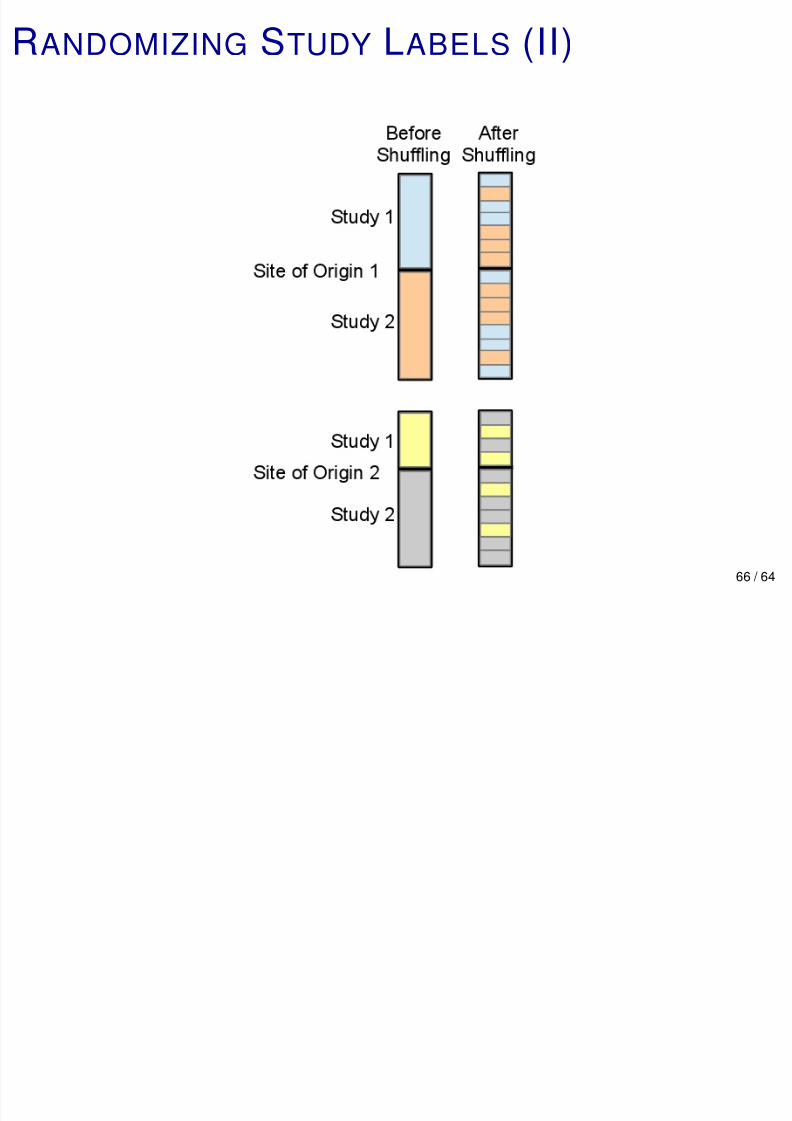
Goal: Quantify how much batch/study effects reduce

accuracy, MCCA.

Randomize study labels within each phenotype .

After shuffling study labels: Accuracy = 98.6%, MCCA =

96.1%.

∼ 8 points of MCCA lost to batch/study effects.

65 / 64

RANDOMIZING STUDY LABELS (II)



66 / 64

CONCLUSIONS



Accuracy should be demonstrated cross-study .

Sample diversity is more important than sample size .

67 / 64

Lecture 7 (D. Geman)

Documents

Transcript of Lecture 7 (D. Geman)