Lecture 6

The Chinagro agricultural supply model

at county level

P.J. Albersen

Presentation available:www.sow.vu.nl/downloadables.htm

Introduction

From the welfare model and the transportation analysis county specific prices and farm profits for the farm/land constraint activities can be calculated.

We seek for the farm decisions at county level a closed form .

Why?

We want to exploit site (county) specific information Due to the number of counties optimization is

'expensive' and cumbersome

Profit maximization problem

We distinguish between inputs (inflows) andoutputs (outflows) , of commodity k in county s, at given prices and , respectively. is the transformation function. are the local endowments.

ks ksk ks ks ks ks ksy ,y 0

s ks ks s

max p y p y

subject to

F ( y y ,e ) 0

ksy

ksy

kspksp

sFse

(1)

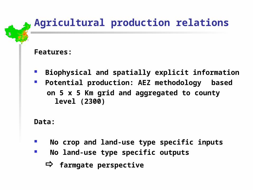
Agricultural production relations

Features:

Biophysical and spatially explicit information Potential production: AEZ methodology based

on 5 x 5 Km grid and aggregated to county level (2300)

Data:

   No crop and land-use type specific inputs   No land-use type specific outputs

farmgate perspective

Revenue index for county s (index dropped):

is a CES - output index (requirements: CRTS, strictly quasiconvex increasing)

Profit maximizing supply of crop k:

Revenue

jjk j j

k

( p )y ( p , y ) y

p

jkkj jkky 0

j j1 jK

( p ) max p y

subject to

h ( y ,..., y ) 1

j( p )

jh

(2)

Aggregate output (1)

Three activities are distinguished at this level irrigated land use rainfed land use grazing

Two inputs are distinguished:1. fertilizer (irrigated and rainfed) or

locally available animal feed (grazing)2. operating capacity

jf

j

Profit maximization for the aggregate output with respect to labor allocation and fertilizer demand is:

and are the prices and L is total labor

j j jf , 0 j j j j j f j j

j j j

max A y ( f , ) p A f

subject to

A L (p )

Aggregate output (2)

fp

(3)

p

0

1

0 10 20 30

Input

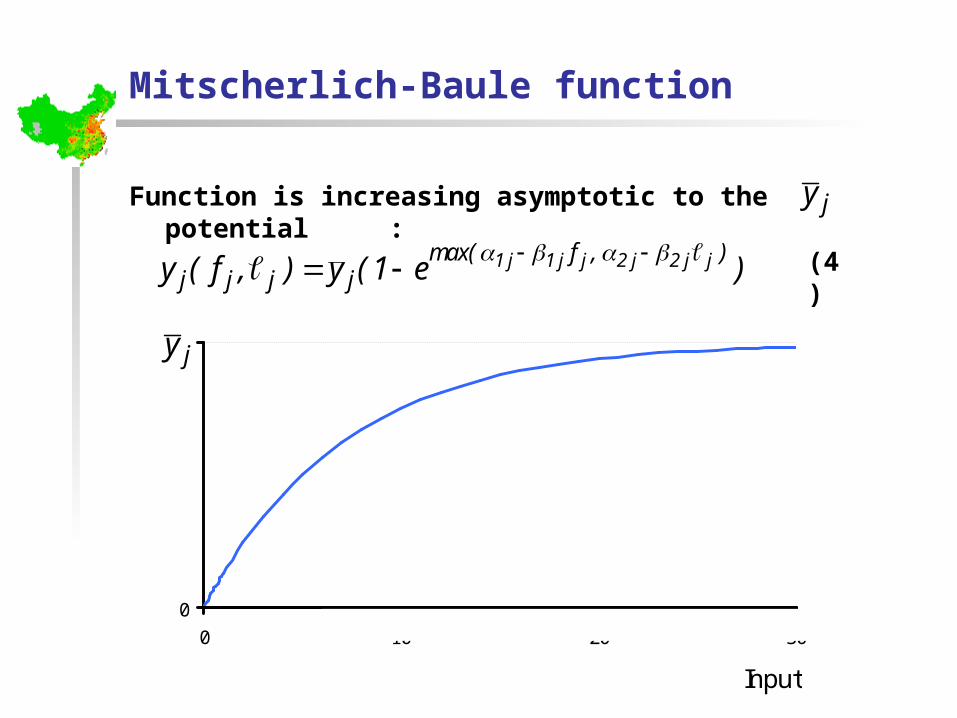
Mitscherlich-Baule function

Function is increasing asymptotic to the potential :

1 j 1 j j 2 j 2 j jmax( f , )j j j jy ( f , ) y (1 e )

jy

jy

(4)

Undefined

No cropping

Single cropping

Limited double cropping

Double cropping

Double cropping with rice

Double rice cropping

Tripple cropping

Tripple rice cropping

Water

Multiple cropping zones under irrigation conditions.

Undefined

Not arable

< 1.2

1.2 - 2.4

2.4 - 3.6

3.6 - 4.8

4.8 - 6.0

6.0 - 7.2

7.2 - 8.4

8.4 - 9.6

9.6 -10.8

10.8 -12.0

12.0 -13.2

13.2 -14.4

14.4 -15.6

15.6 -16.8

> 16.8

Water

Annual potential production (tons/ha), weighted average of irrigation and rain-fed potentials.

No resource wasted

In optimum no resource will be wasted and both input effects are equal.

Fertilizer can be written as a linear relation of labor:

For the optimal situation the production function can be expressed in the local resource operating capacity:

2 j 1 j 2 jj j

1 j 1 jf

2 j 2 j jj j jy ( ) y (1 e )

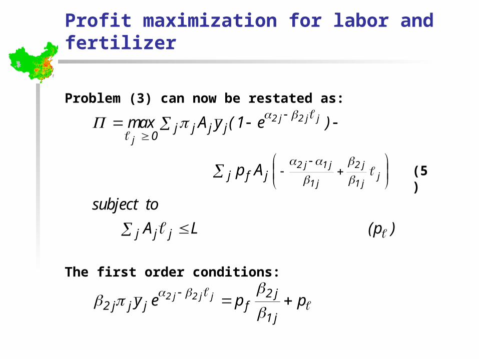
Problem (3) can now be restated as:

The first order conditions:

2 j 2 j j

j

2 j 1 j 2 jj

1 j 1 j

j j j j 0

j f j

j j j

max A y (1 e )

p A

subject to

A L (p )

Profit maximization for labor and fertilizer

2 j 2 j j 2 j2 j j j f

1 jy e p p

(5)

Labor demand and wage rate

Without iteration we can solve the labour demand:

and derive the wage rate:

in closed form.

j 2 j f 2 j j j2 j 2 j

1 1ln( p p ) ln( y )

jj jj 2 j 2 j j j

2 jf

jj

2 j

AA ln( y ) L

p exp pA