LECTURE 6: INTERIOR POINT METHOD 1. Motivation 2. Basic concepts 3. Primal affine scaling algorithm 4. Dual affine scaling algorithm

Motivation • Simplex method works well in general, but suffers from

exponential-time computational complexity. • Klee-Minty example shows simplex method may have to

visit every vertex to reach the optimal one. • Total complexity of an iterative algorithm = # of iterations x # of operations in each iteration • Simplex method - Simple operations: Only check adjacent extreme points - May take many iterations: Klee-Minty example Question: any fix?

Complexity of the simplex method

Worst case performance of the simplex method Klee-Minty Example: • Victor Klee, George J. Minty, “How good is the simplex

algorithm?’’ in (O. Shisha edited) Inequalities, Vol. III (1972), pp. 159-175.

Klee-Minty Example

Klee-Minty Example

Karmarkar’s (interior point) approach • Basic idea: approach optimal solutions from the interior of the feasible domain

• Take more complicated operations in each iteration to find a better moving direction

• Require much fewer iterations

General scheme of an interior point method

• An iterative method that moves in the interior of the feasible domain

Interior movement (iteration) • Given a current interior feasible solution , we have

> 0 An interior movement has a general format

Key knowledge • 1. Who is in the interior? - Initial solution • 2. How do we know a current solution is optimal? - Optimality condition • 3. How to move to a new solution? - Which direction to move? (good feasible direction) - How far to go? (step-length)

Q1 - Who is in the interior? • Standard for LP

• Who is at the vertex? • Who is on the edge? • Who is on the boundary? • Who is in the interior?

What have learned before

Who is in the interior? • Two criteria for a point x to be an interior feasible solution:

1. Ax = b (every linear constraint is satisfied) 2. x > 0 (every component is positive)

• Comments: 1. On a hyperplane , every point is interior relative to H. 2. For the first orthant K = , only those x > 0 are interior relative to K.

Example

How to find an initial interior solution? • Like the simplex method, we have

- Big M method - Two-phase method (to be discussed later!)

Key knowledge • 1. Who is in the interior? - Initial solution • 2. How do we know a current solution is optimal? - Optimality condition • 3. How to move to a new solution? - Which direction to move? (good feasible direction) - How far to go? (step-length)

Q2 - How do we know a current solution is optimal? • Basic concept of optimality: A current feasible solution is optimal if and only if “no feasible direction at this point is a good direction.”

• In other words, “every feasible direction is not a good

direction to move!”

Feasible direction • In an interior-point method, a feasible direction at a current solution is a direction that allows it to take a small movement while staying to be interior feasible. • Observations: - There is no problem to stay interior if the step-length is small enough. - To maintain feasibility, we need

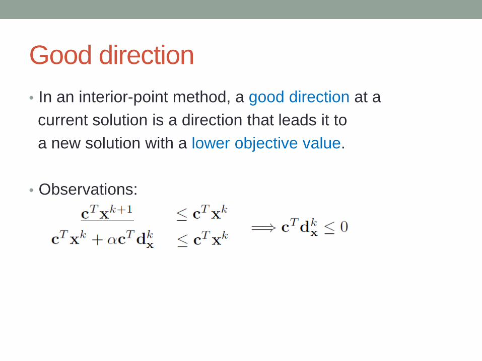
Good direction • In an interior-point method, a good direction at a current solution is a direction that leads it to a new solution with a lower objective value. • Observations:

Optimality check • Principle: “no feasible direction at this point is a good direction.”

Key knowledge • 1. Who is in the interior? - Initial solution • 2. How do we know a current solution is optimal? - Optimality condition • 3. How to move to a new solution? - Which direction to move? (good feasible direction) - How far to go? (step-length)

Q3 – How to move to a new solution? 1. Which direction to move? - a good, feasible direction “Good” requires “Feasible” requires

Question: any suggestion?

A good feasible direction • Reduce the objective value

• Maintain feasibility

Projection mapping • A projection mapping projects the negative gradient vector

–c into the null space of matrix A

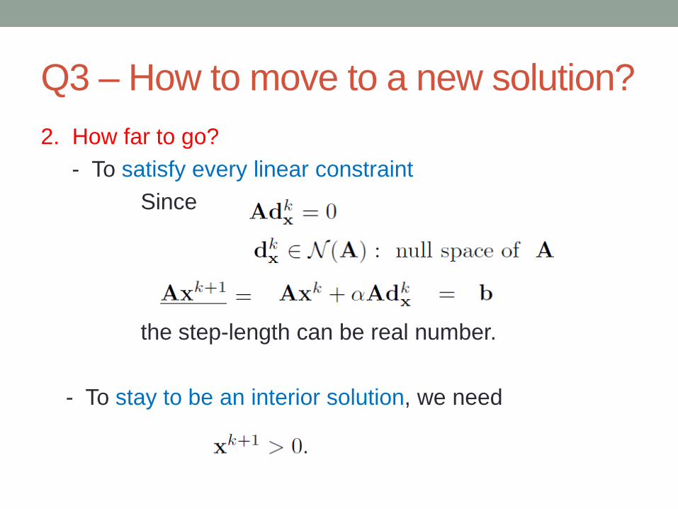
Q3 – How to move to a new solution? 2. How far to go? - To satisfy every linear constraint Since

the step-length can be real number.

- To stay to be an interior solution, we need

How to choose step-length? • One easy approach - in order to keep > 0 we may use the “minimum ratio test” to determine the step-length. Observation: - when is close to the boundary, the step-length may be very small. Question: then what?

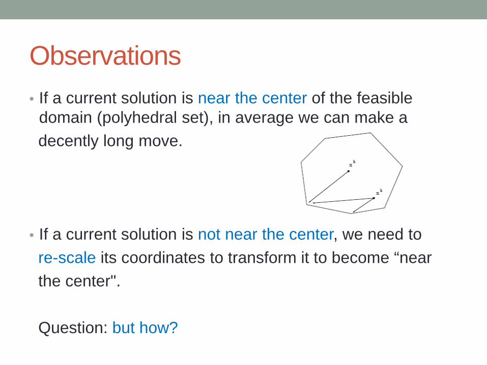
Observations • If a current solution is near the center of the feasible

domain (polyhedral set), in average we can make a decently long move.

• If a current solution is not near the center, we need to re-scale its coordinates to transform it to become “near the center". Question: but how?

Where is the center? • We need to know where is the “center” of the non-negative/first orthant . -Concept of equal distance to the boundary Question: If not, what to do?

Concept of scaling • Scale • Define a diagonal scaling matrix

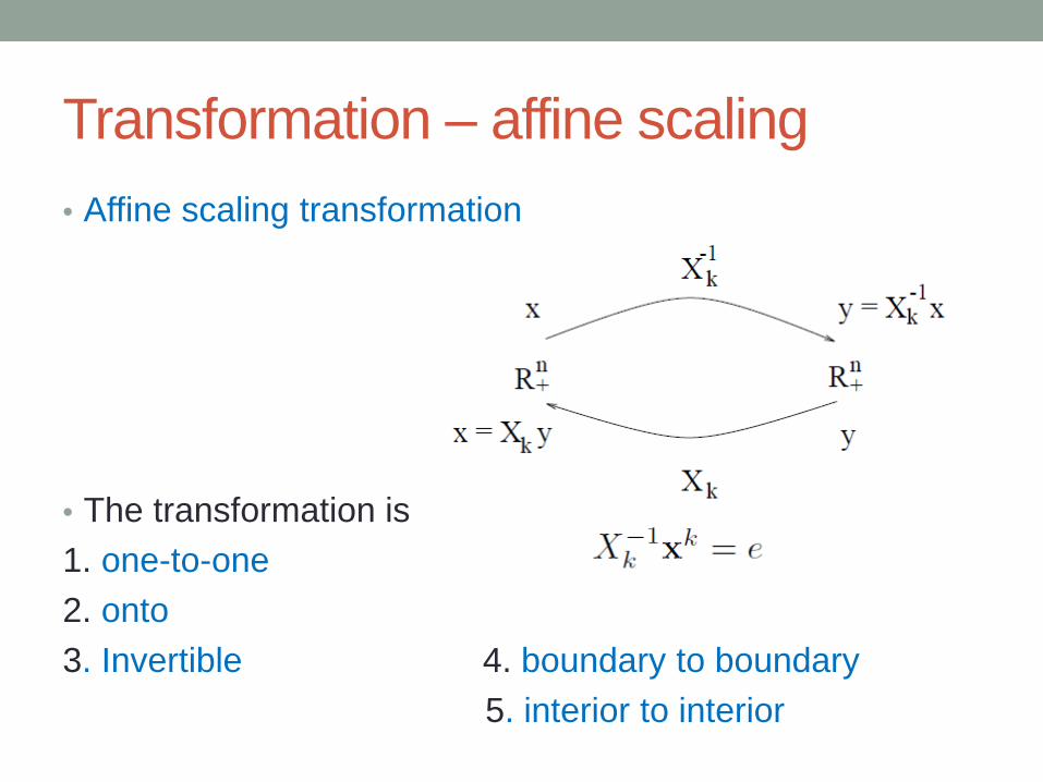
Transformation – affine scaling • Affine scaling transformation

• The transformation is 1. one-to-one 2. onto 3. Invertible 4. boundary to boundary 5. interior to interior

Transformed LP

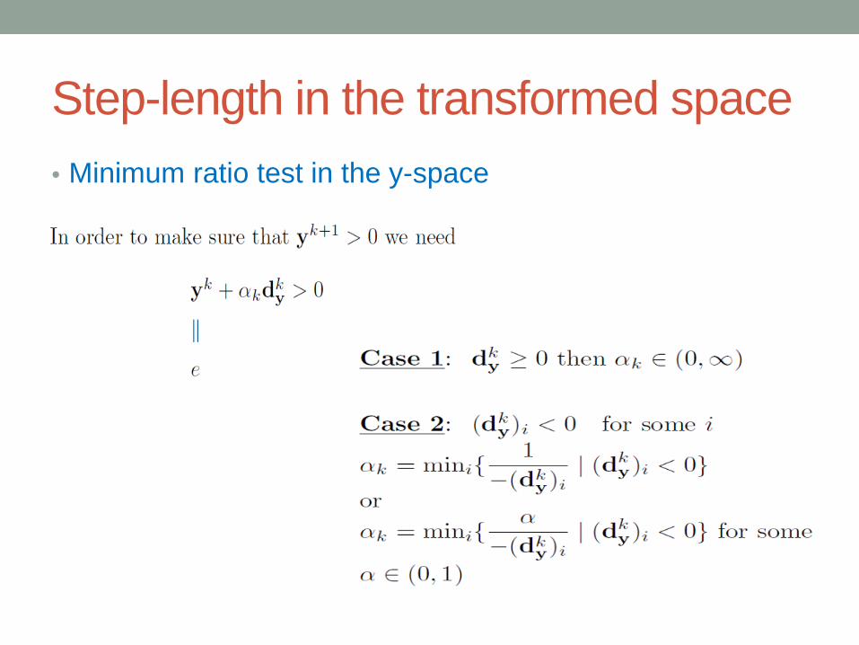
Step-length in the transformed space • Minimum ratio test in the y-space

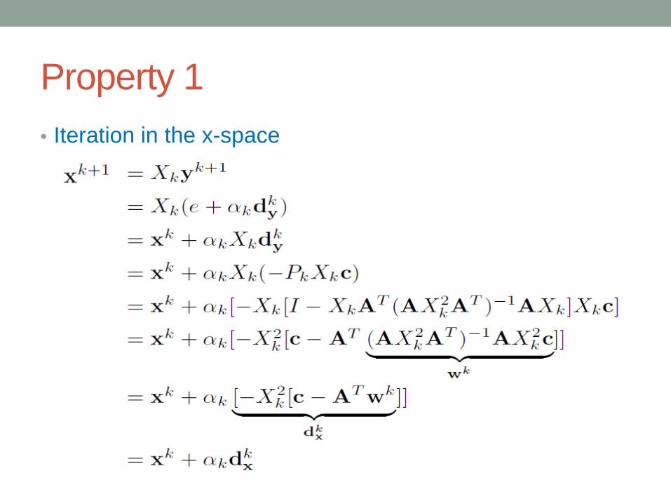
Property 1 • Iteration in the x-space

Property 2 • Feasible direction in x-space

Property 3 • Good direction in x-space

Property 4 • Optimality check (Lemma 7.2)

Property 5 • Well-defined iteration sequence (Lemma 7.3)

From properties 3 and 4, if the standard form LP is bounded below and is not a constant, then the sequence is well-defined and strictly decreasing.

Property 6 • Dual estimate, reduced cost and stopping rule We may define

Property 7 • Moving direction and reduced cost

Primal affine scaling algorithm

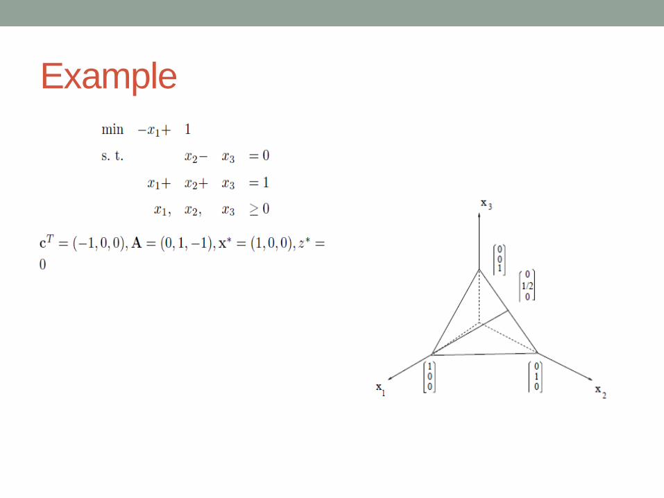
Example

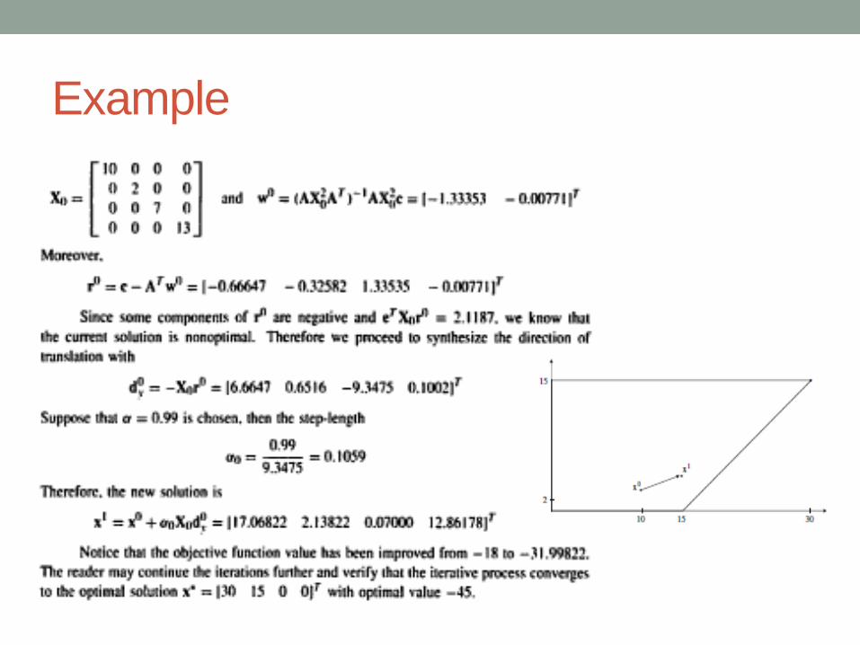
Example

How to find an initial interior feasible solution?

• Big-M method Idea: add an artificial variable with a big penalty (big-M)

• Objective

Properties of (big-M) problem (1) It is a standard form LP with n+1 variables and m constraints.

(2) e is an interior feasible solution of (big-M).

(3)

Two-phase method

Properties of (Phase-I) problem

Facts of the primal affine scaling algorithm

More facts

Improving performance – potential push • Idea: (Potential push method) - Stay away from the boundary by adding a potential push. Consider Use

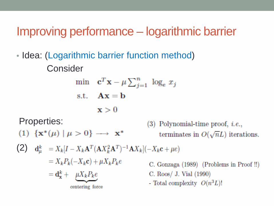
Improving performance – logarithmic barrier

• Idea: (Logarithmic barrier function method) Consider Properties: (2)

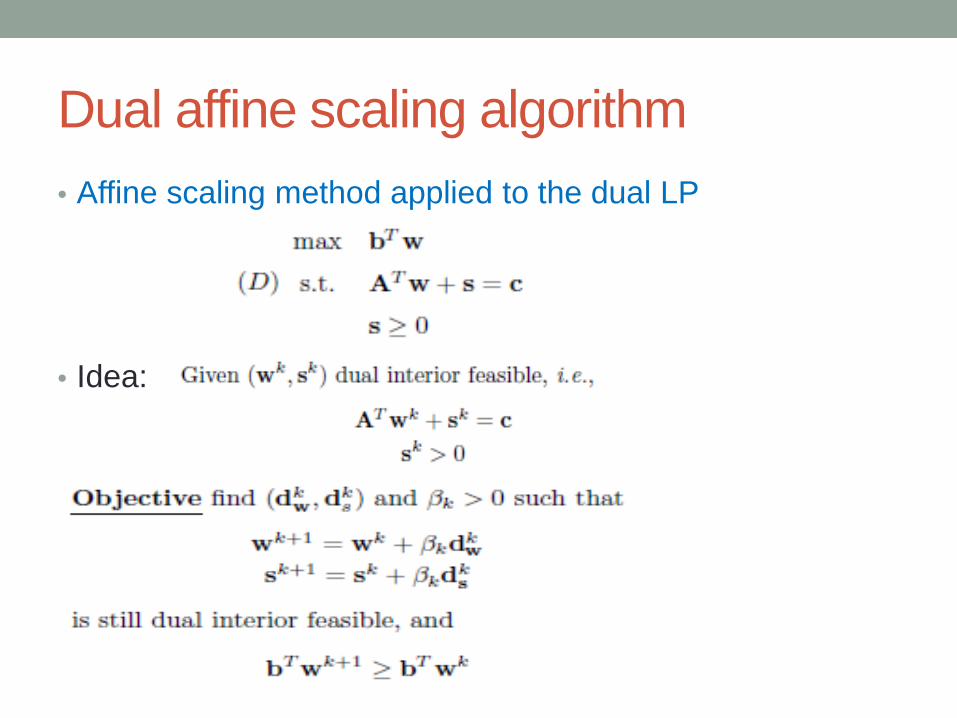
Dual affine scaling algorithm • Affine scaling method applied to the dual LP

• Idea:

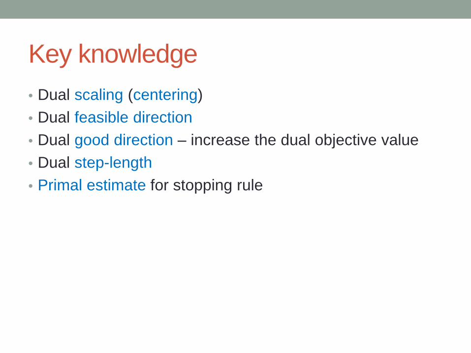
Key knowledge • Dual scaling (centering) • Dual feasible direction • Dual good direction – increase the dual objective value • Dual step-length • Primal estimate for stopping rule

Observation 1 • Dual scaling (centering)

Observation 2 • Dual feasibility (feasible direction)

Observation 3 • Increase dual objective function (good direction)

Observation 4 • Dual step-length

Observation 5 • Primal estimate We define

Dual affine scaling algorithm

Find an initial interior feasible solution

Properties of (big-M) problem

Performance of dual affine scaling • No polynomial-time proof ! • Computational bottleneck • Less sensitive to primal degeneracy and numerical errors, but sensitive to dual degeneracy. • Improves dual objective value very fast, but attains primal feasibility slowly.

Improving performance 1. Logarithmic barrier function method

Polynomial-time proof

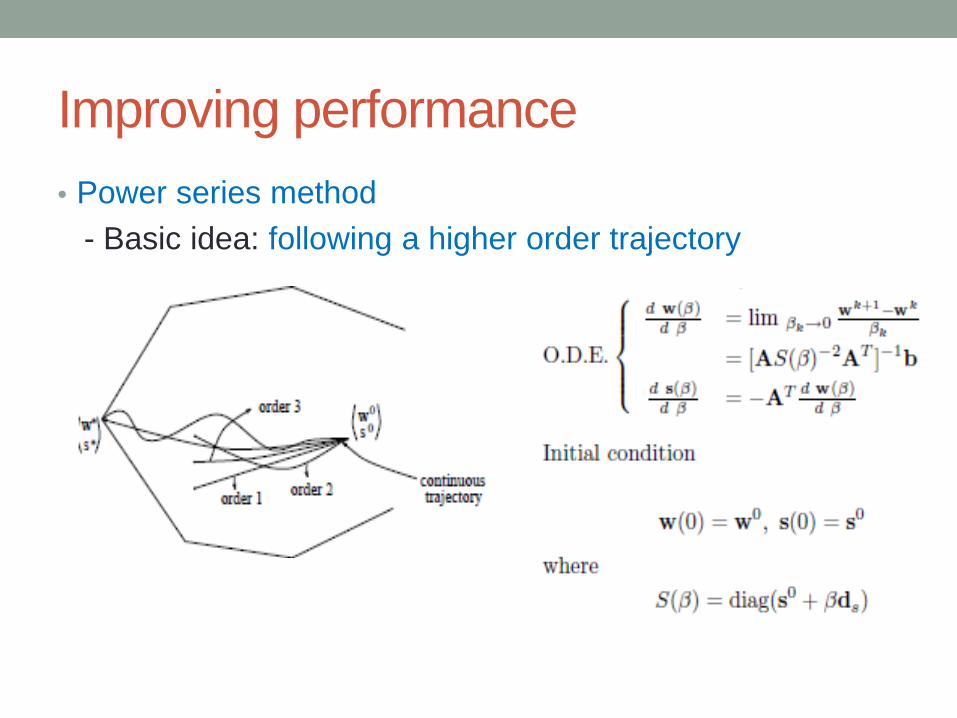
Improving performance • Power series method - Basic idea: following a higher order trajectory

Power series expansion

Karmarkar’s projective scaling algorithm • Karmarkar’s standard form

Terminologies • Feasible solution

• Interior feasible solution

Basic assumptions

Example

Where is the center? • 3-dimensional

• n-dimensional

How far away from center to boundaries?

How to rescale interior to center?

Example

Properties of projective scaling

Karmarkar’s algorithm

Karmarkar’s algorithm

Kramarkar’s algorithm

Choice of step length

Example

Example

Performance analysis

Performance analysis