Lecture 5

(v) Adaptive step length for Runge Kutta

One step methods can easily be modified to vary the step length �t as the function uvaries in order to account for how rapidly or slowly the solution u is varying with time.There are a number of commonly used adaptive schemes, the underlying principle isto use knowledge of how the error depends on �t to help estimate whether the errormay be increasing beyond some pre-set tolerance (and so smaller time steps shouldbe used), or whether errors are su�ciently below a tolerance that the step size canbe increased.

As an example of one adaptive method, consider the Runge-Kutta fourth ordermethod given above, (4.47)-(4.51), denoted RK4. The background theory is thatwhen using RK4 there will be some constants K

1

, K2

, K3

, such that

Trunction error Tn

⇠ K1

(�t)4u(v) (5.1)

Local error |en

| ⇠ K2

�t|Tn

| (5.2)

so |en

| ⇠ K3

(�t)5u(v). (5.3)

Suppose we are at tn

and want to use a step �tn

1. apply RK4 over step �tn

to get value Ua

where

Ua

= un+1

+(�t

n

)5u(v)

5!+O(�t6

n

) (5.4)

2. apply RK4 twice over step �tn

/2 to get value Ub

Ub

= un+1

+2(�t

n

2

)5u(v)

5!+O(�t6

n

) (5.5)

Then

Ua

� Ub

⇠ 15

16

u(v)

5!(�t

n

)5. (5.6)

Suppose we had used an alternative step �tn

for which this di↵erence would exactlybe a pre-set tolerance, that is

tolerance =15

16

u(v)

5!(�t

n

)5. (5.7)

Thus we can remove the unknown fifth-derivative of u by dividing these expressions✓

�tn

�tn

◆

5

=tolerance

Ua

� Ub

, (5.8)

31

or

�tn

=

✓

tolerance

Ua

� Ub

◆

1/5

�tn

, (5.9)

and this gives an algorithm for adapting the step length: if (5.9) gives a step lengthwhich is less than �t

n

, then we repeat the step from tn

with the reduced step length,if (5.9) gives an increased step length, we use that step as �t

n+1

and the valueUn+1

= Ub

at tn+1

. Of course we have to do more work each step since we e↵ectivelyapply RK4 three times.

Algorithm: User provides start time, end time, tolerance.

1. Set TOL=tolerance

2. Set t0

as start time, �t0

as first step length and n = 0

3. while tn

end time

(a) apply RK4 with step �tn

to determine Ua

and twice with step �tn

/2 tocalculate U

b

(b) if |Ua

� Ub

| >TOL, step fails, set

�tn

=

✓

TOL

|Ua

� Ub

|◆

1/5

�tn

(5.10)

and go back to (a). (This reduces the step and repeats.)

else |Ua

� Ub

| TOL, set

�tn+1

=

✓

TOL

|Ua

� Ub

|◆

1/5

�tn

(5.11)

Un+1

= Ub

tn+1

= tn

+�tn

n = n+ 1

(this increases the step length for next step).

end while

As we have been dealing with local error the lengthening of step can be misleading,the global error has order (�t)4 so in (5.11) above we can use as an alternative

�tn+1

=

✓

TOL

|Ua

� Ub

|◆

1/4

�tn

. (5.12)

32

This is more robust in practice. It is also good practice to set some minimum steplength and to alert a user if the predicted step length becomes too small, usuallystopping the integration from continuing. We will look at implementing this adaptivealgorithm in the routine rk4a.m.

The adaptation method above is only one of a number that are widely used. Anotherstrategy is to use the flexibility inherent in Runge-Kutta families of solutions toproduce increments with di↵erent order of magnitude but using the same time pointswithin the step from t

n

to tn+1

and then to use the di↵erence between the estimatesto control step length.

In the matlab ode23 family, a second and a third order method is used. The Butchertable is modified slightly so as to have two rows at the bottom showing coe�cents forthe two di↵erent order estimates of the increment. The Butcher table is:

0 11/2 1/23/4 0 3/41 2/9 3/9 4/9

2/9 3/9 4/911/72 30/72 40/72 �9/72

For this routine, a second order estimate for the update is

Ua

= U(n) +�t

9(2k

1

+ 3k2

+ 4k3

),

and this value is used to evaluate k4

at time tn

+�t, and then a third order estimatefor the update is

Ub

= Un

+�t

72(11k

1

+ 30k2

+ 40k3

� 9k4

).

With these two estimates, one might crudely say Ua

= un

+ O(�t2) and Ub

⇡ un

sothat the di↵erence U

a

�Ub

can be used as a measure of accuracy and by introducinga tolerance, the step length reduced if the di↵erence is too large or increased if thedi↵erence is smaller than the tolerance. This is illustrated in the course matlab routinerk23a.m and is the basis of the ode23 family of routines in matlab.

The same idea can be applied using a fourth and fifth order comparison, this is usedfor ode45 in matlab. It is based on a method by Dormand and Prince. In this casethere are seven calculations to estimate the tangent, f , and the Butcher table is:

33

0 1

1/5 1/5

3/10 3/40 9/40

4/5 44/45 �56/15 32/9

8/9 19372/6561 �25360/2187 64448/6561 �212/729

1 9017/3168 �355/33 46732/5247 49/176 �5103/18656

1 35/384 0 500/1113 125/192 �2187/6784 11/84

c

r

35/384 0 500/1113 125/192 �2187/6784 11/84 0

d

r

5179/57600 0 7571/16695 393/640 �92097/339200 187/2100 1/40

As with the 2-3 method, we calculate a fourth order estimate,

Ua

= Un

+�t(c1

⇤ k1

+ c2

⇤ k2

+ c3

⇤ k3

+ c4

⇤ k4

+ c5

⇤ k5

+ c6

⇤ k6

),

and a fifth order estimate

Ub

= Un

+�t(d1

⇤ k1

+ d2

⇤ k2

+ d3

⇤ k3

+ d4

⇤ k4

+ d5

⇤ k5

+ d6

⇤ k6

+ d7

⇤ k7

),

and use the di↵erence Ua

�Ub

as an indicator of the error in the step, again repeatingthe step with a decreased step size if this di↵erence is greater than some pre-settolerance, and increasing the next time step length if the di↵erence is less that thetolerance. One way of doing this is shown in the course routine rk45a.m but it is alsothe basis for ode45 in matlab.

Semi-implicit methods: Predictor-Corrector

All implicit methods will in principle require solution of a non-linear equation (orsystem) at each time step. A version of Newton iteration can be used so that withinthe time stepping sequence, there is another iteration that provides convergence ofthe Newton iteration. A drawback with Newton iteration is that the derivative (or fora system, the Jacobian) of the function f is required, this may be known analyticallyor it may be approximated numerically but this can be a significant problem. Alter-native methods for implicit schemes, which are a variant on fixed point methods, andwhich do not require evaluation of a derviative or Jacobian matrix are often labelledpredictor-corrector or semi-implicit schemes These usually combine an explicit ‘pre-dictor’ step with a semi-implicit iteration even if the latter is only one step and nottaken to convergence.

As an example of this idea, consider a fully implicit Euler method

Un+1

= Un

+�tf(tn+1

, Un+1

), (5.13)

where Un

is the computed value at tn

. Then an explicit predictor for the value Un+1

is

U (0)

n+1

= Un

+�tf(tn

, Un

), (5.14)

34

and this allows a corrector step which uses this value in the implicit formula,

Un+1

= Un

+�tf(tn+1

, U (0)

n+1

). (5.15)

Alternately, the predictor step can be used to give an initial value for a fixed pointiteration where iterates are successively calculated by

U (k+1)

n+1

= Un

+�tf(tn+1

, U (k)

n+1

) k = 0, 1, 2, . . . , (5.16)

until |U (k+1)

n+1

� U (k)

n+1

| is less than a predefined tolerance.

Another fixed point iteration might be based on Improved Euler (or the trapezoidalrule), so that

U (k+1)

n+1

= Un

+1

2�t

h

f(tn

, Un

) + f(tn+1

, U (k)

n+1

)i

k = 0, 1, 2, . . . , (5.17)

again, until |U (k+1)

n+1

� U (k)

n+1

| is less than a predefined tolerance.

Example: Van der Pol oscillator

A Van der Pol oscillator is an example of a second order system, essentially an oscil-lator with non-linear damping, which with no forcing is described by

u00 + ↵(u2 � 1)u0 + u = 0 (5.18)

u(0) = u0

, (5.19)

u0(0) = v0

, (5.20)

or as a second order system

u0 = v, u(0) = u0

, (5.21)

v0 = �u� ↵(u2 � 1)v, v(0) = v0

. (5.22)

This is a modification of the simple spring and mass we considered at the start ofthis lecture, reducing to the same equations when ↵ = 0 and like that system, has alimit cycle behaviour in (u, v) space. In the matlab code vanderpol.m we use threealgorithms, explicit Euler, improved Euler and implicit Euler using a predictor stepto give an initial value for a fixed point iteration. In each case we use the initialconditions u

0

= 2, v0

= 0.

If we set ↵ = 0, then a computed solution is illustrated in Figure 4 where as should beexpected now, the explicit scheme results in a growing solution, the implicit schemedecays and while Improved Euler appears to conserve the solution correctly, it alsohas a discrete solution where u2 + v2 is increasing very slowly.

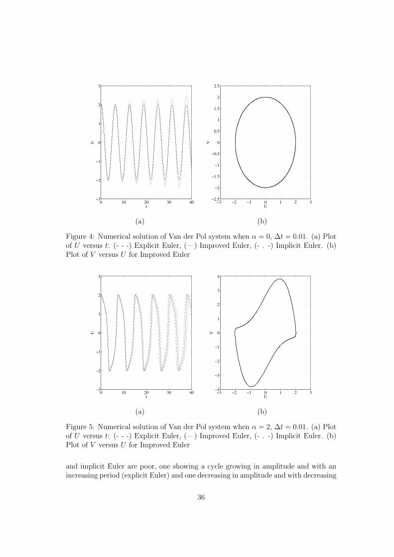
Setting ↵ > 0 brings in the non-linear term, example calculations for ↵ = 2 withthe same time step, �t = 0.01 are shown in Figure 5 where both first order explicit

35

0 10 20 30 40−3

−2

−1

0

1

2

3

t

U

−3 −2 −1 0 1 2 3−2.5

−2

−1.5

−1

−0.5

0

0.5

1

1.5

2

2.5

UV

(a) (b)

Figure 4: Numerical solution of Van der Pol system when ↵ = 0, �t = 0.01. (a) Plotof U versus t: (- - -) Explicit Euler, (—) Improved Euler, (- . -) Implicit Euler. (b)Plot of V versus U for Improved Euler

0 10 20 30 40−3

−2

−1

0

1

2

3

t

U

−3 −2 −1 0 1 2 3−4

−3

−2

−1

0

1

2

3

4

U

V

(a) (b)

Figure 5: Numerical solution of Van der Pol system when ↵ = 2, �t = 0.01. (a) Plotof U versus t: (- - -) Explicit Euler, (—) Improved Euler, (- . -) Implicit Euler. (b)Plot of V versus U for Improved Euler

and implicit Euler are poor, one showing a cycle growing in amplitude and with anincreasing period (explicit Euler) and one decreasing in amplitude and with decreasing

36

0 10 20 30 40−3

−2

−1

0

1

2

3

t

U

−3 −2 −1 0 1 2 3−4

−3

−2

−1

0

1

2

3

4

U

V

(a) (b)

Figure 6: Numerical solution of Van der Pol system when ↵ = 0, �t = 0.001. (a)Plot of U versus t: (- - -) Explicit Euler, (—) Improved Euler, (- . -) Implicit Euler.(b) Plot of V versus U for Improved Euler

period (implicit Euler). In part (b) of the figure the phase plot of Improved Eulershows that periodicity is being preserved by the method.

Of course, one can improve the performance of a first order scheme by decreasing thetime step, and in Figure 6, the solution appears much better.

However, if this integration is carried on to longer itmes, the solution for the two firstorder methods remains problematic, see Figure 7

It is also worth observing that for the linear system with the two first order dis-cretisations, both theory and the computations show that growth (explicit) or decay(implicit) are exponential, yet in the non-linear system, while the oscillation periodshows very slow change, the amplitude does not appear to grow exponentially.

37

360 370 380 390 400−3

−2

−1

0

1

2

3

t

U

−4 −2 0 2 4−4

−3

−2

−1

0

1

2

3

4

U

V

(a) (b)

Figure 7: Numerical solution of Van der Pol system when ↵ = 0, �t = 0.001 atlonger time. (a) Plot of U versus t: (- - -) Explicit Euler, (—) Improved Euler, (- . -)Implicit Euler. (b) Plot of V versus U for Improved Euler

38