Lecture 5: Stochastic Runge Kutta Methods - Aaltossarkka/course_s2014/handout5.pdf · Lecture 5:...
45
Lecture 5: Stochastic Runge–Kutta Methods Arno Solin Aalto University, Finland November 25, 2014 Arno Solin (Aalto) Lecture 5: Stochastic Runge–Kutta Methods November 25, 2014 1 / 50
Transcript of Lecture 5: Stochastic Runge Kutta Methods - Aaltossarkka/course_s2014/handout5.pdf · Lecture 5:...

Lecture 5: Stochastic Runge–Kutta Methods
Arno Solin
Aalto University, Finland
November 25, 2014
Arno Solin (Aalto) Lecture 5: Stochastic Runge–Kutta Methods November 25, 2014 1 / 50

Contents
1 Introduction
2 Runge–Kutta methods for ODEs
3 Strong stochastic Runge–Kutta methods
4 Weak stochastic Runge–Kutta methods
5 Summary
Arno Solin (Aalto) Lecture 5: Stochastic Runge–Kutta Methods November 25, 2014 2 / 50

Overview of this lecture
Runge–Kutta methods for ODEsTaylor series.General Runge–Kutta schemes.Explicit and implicit schemes.
Strong stochastic Runge–Kutta methodsItô–Taylor series.A family of strong order 1.0 schemes.The iterated Itô integrals.
Weak stochastic Runge–Kutta methodsA family of weak order 2.0 schemes.Approximating the iterated Itô integrals.
Arno Solin (Aalto) Lecture 5: Stochastic Runge–Kutta Methods November 25, 2014 4 / 50
Runge–Kutta: Basic principles
A family of iterative methods for solving differential equations.Based on Taylor series (see the previous lecture), ...... but are derivative-free.Plug-and-play methods that only requires specification of thedifferential equation (at least ideally).There are other methods as well (not considered here):
Multistep methods (e.g. Adams methods)Multiderivative methodsHigher-order methods (e.g. Nyström method)Tailored methods (for specific problems)
Arno Solin (Aalto) Lecture 5: Stochastic Runge–Kutta Methods November 25, 2014 6 / 50
Runge–Kutta: Motivation
Consider a first-order non-linear ODE
dx(t)dt
= f(x(t), t), x(t0) = given,
The simplest Runge–Kutta method is the (forward) Euler scheme.It is based on sequential linearization of the ODE system:
x(tk+1) = x(tk ) + f(x(tk ), tk ) ∆t .
Easy to understand and implement.The global error of the method depends linearly onthe step size ∆t .
Arno Solin (Aalto) Lecture 5: Stochastic Runge–Kutta Methods November 25, 2014 7 / 50

Taylor series [1/2]
The ODE system can be integrated to give
x(t) = x(t0) +
∫ t
t0f(x(τ), τ) dτ.
Recall from the previous lecture that we used a Taylor seriesexpansion for the solution of the ODE
x(t) = x(t0) + f(x(t0), t0) (t − t0)
+12!L f(x(t0), t0) (t − t0)2
+13!L2 f(x(t0), t0) (t − t0)3 + . . .
We used the linear operator
L(•) =∂
∂t(•) +
∑i
fi∂
∂xi(•)
Arno Solin (Aalto) Lecture 5: Stochastic Runge–Kutta Methods November 25, 2014 8 / 50

Taylor series [2/2]
In other words, the series expansion is equal to
x(t) = x(t0) + f(x(t0), t0) (t − t0)
+12!
{∂
∂tf(x(t0), t0) +
∑i
fi(x(t0), t0)∂
∂xif(x(t0), t0)
}(t − t0)2
+13!
{∂[L f(x(t0), t0)]
∂t+∑
i
fi(x(t0), t0)∂[L f(x(t0), t0)]
∂xi
}(t − t0)3
+ . . .
If we were only to consider the terms up to ∆t , we would recoverthe Euler method.
Arno Solin (Aalto) Lecture 5: Stochastic Runge–Kutta Methods November 25, 2014 9 / 50

Derivation of a higher-order method [1/4]
However, here we wish to get hold of higher-order methods.For the sake of simplicity, we now stop at the term(t − t0)2 = (∆t)2.We get
x(t0 + ∆t) ≈ x(t0) + f(x(t0), t0) ∆t
+12
{∂
∂tf(x(t0), t0) +
∑i
fi(x(t0), t0)∂
∂xif(x(t0), t0)
}(∆t)2.
We aim to get rid of the derivatives and be able to write theexpression in terms of the function f(·, ·) evaluated at variouspoints.
Arno Solin (Aalto) Lecture 5: Stochastic Runge–Kutta Methods November 25, 2014 10 / 50

Derivation of a higher-order method [2/4]
We now seek a form with an extra stage:
x(t0 + ∆t) ≈ x(t0) + A f(x(t0), t0) ∆t+ B f(x(t0) + C f(x(t0), t0) ∆t , t0 + D ∆t) ∆t ,
where A,B,D, and D are unknown.In the last term, we can consider the truncated Taylor expansion(linearization) around f(x(t0), t0) with the chosen increments asfollows:
f(x(t0) + C f(x(t0), t0) ∆t , t0 + D ∆t) = f(x(t0), t0)
+ C(∑
i
fi(x(t0), t0)∂
∂xif(x(t0), t0)
)∆t + D
∂f(x(t0), t0)
∂t∆t + · · ·
Arno Solin (Aalto) Lecture 5: Stochastic Runge–Kutta Methods November 25, 2014 11 / 50

Derivation of a higher-order method [3/4]
Combining the previous two equations gives:
x(t0 + ∆t) ≈ x(t0) + (A + B) f(x(t0), t0) ∆t
+ B[C∑
i
fi(x(t0), t0)∂
∂xif(x(t0), t0) + D
∂f(x(t0), t0)
∂t
](∆t)2.
If we now compare the above equation to the original truncatedTaylor expansion, we get the following conditions for ourcoefficients:
A + B = 1, B =12, C = 1, and D = 1.
Arno Solin (Aalto) Lecture 5: Stochastic Runge–Kutta Methods November 25, 2014 12 / 50
Derivation of a higher-order method [4/4]
We derived here is a two-stage method (known as Heun’smethod):
x(t0 + ∆t) = x(t0) +∆t2{
f(x1, t0) + f(x2, t0 + ∆t)},
where the supporting values are given by
x1 = x(t0),
x2 = x(t0) + f(x1, t0) ∆t .
The method (in practice the finite differences) are determined bythe choices we did in truncating the series expansion.This method is of order 2.
Arno Solin (Aalto) Lecture 5: Stochastic Runge–Kutta Methods November 25, 2014 13 / 50

A general Runge–Kutta method
Algorithm: Runge–Kutta methodStart from x(t0) = x(t0) and divide the integration interval [t0, t ] into nsteps t0 < t1 < t2 < . . . < tn = t such that ∆t = tk+1 − tk . Theintegration method is defined by its Butcher tableau:
c A
αT
On each step k approximate the solution as follows:
x(tk+1) = x(tk ) +s∑
i=1
αi f(xi , ti) ∆t ,
where ti = tk + ci∆t and xi = x(tk ) +∑s
j=1 Ai,j f(xj , tj) ∆t .
Arno Solin (Aalto) Lecture 5: Stochastic Runge–Kutta Methods November 25, 2014 14 / 50

Butcher tableau
Ordinary Runge–Kutta methods are commonly expressed in termsof a table called the Butcher tableau:
c1 A1,1c2 A2,1 A2,2...
.... . .
cs As,1 As,2 . . . As,sα1 α2 . . . αs
Arno Solin (Aalto) Lecture 5: Stochastic Runge–Kutta Methods November 25, 2014 15 / 50

Example: Forward Euler
Example (Forward Euler)The forward Euler scheme has the Butcher tableau:
0 01
which gives the recursion x(tk+1) = x(tk ) + f(x(tk ), tk ) ∆t .
Arno Solin (Aalto) Lecture 5: Stochastic Runge–Kutta Methods November 25, 2014 16 / 50

Example: RK4
Example (The fourth-order Runge–Kutta method)The well-known RK4 method in Ch. 1 has the following Butchertableau:
012
12
12 0 1
21 0 0 1
16
13
13
16
Arno Solin (Aalto) Lecture 5: Stochastic Runge–Kutta Methods November 25, 2014 17 / 50
Implicit schemes [1/2]
We have considered this far so-called explicit schemes.Numerical instability, when the solution includes rapidly varyingterms (stiff problems).Explicit schemes use very small step sizes in order to not divergefrom a solution path (computationally demanding).In implicit Runge–Kutta methods, the Buther tableau is no longerlower-triangular.On every step, a system of algebraic equations has to be solved(computationally demanding, but more stabile).
Arno Solin (Aalto) Lecture 5: Stochastic Runge–Kutta Methods November 25, 2014 18 / 50
Implicit schemes [2/2]
The simplest implicit method is the backward Euler scheme.
Example (Backward Euler)
The implicit backward Euler scheme has the Butcher tableau:
1 11
which gives the recursion x(tk+1) = x(tk ) + f(x(tk+1), tk + ∆t) ∆t .
Arno Solin (Aalto) Lecture 5: Stochastic Runge–Kutta Methods November 25, 2014 19 / 50

Example [1/2]
We study the two-dimensional non-linear ordinary differentialequation system
x1 = x1 − x2 − x31 ,
x2 = x1 + x2 − x32 ,
Arno Solin (Aalto) Lecture 5: Stochastic Runge–Kutta Methods November 25, 2014 20 / 50
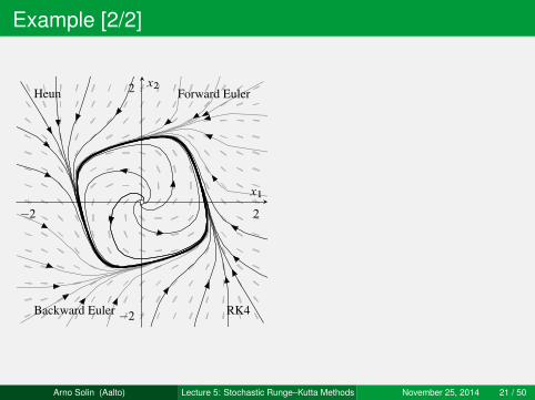
Example [2/2]
Forward EulerHeun
Backward Euler RK4
�2 2
�2
2
x1
x2
Arno Solin (Aalto) Lecture 5: Stochastic Runge–Kutta Methods November 25, 2014 21 / 50

Strong stochastic Runge–Kutta: Basic principles
A family of iterative methods for solving stochastic differentialequations.Based on Itô–Taylor series (see the previous lecture), ...... but are derivative-free.Plug-and-play methods that only requires specification of the driftand diffusion function of the SDE (at least ideally).We divide the methods into strong and weak methods(as we did for the Itô–Taylor series approximations).A word of warning: Stochastic Runge–Kutta methods are not aseasy to grasp as the ordinary ones.
Arno Solin (Aalto) Lecture 5: Stochastic Runge–Kutta Methods November 25, 2014 23 / 50
Itô–Taylor series [1/1]
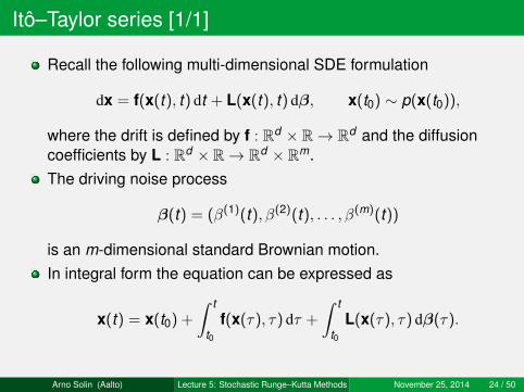
Recall the following multi-dimensional SDE formulation
dx = f(x(t), t) dt + L(x(t), t) dβ, x(t0) ∼ p(x(t0)),
where the drift is defined by f : Rd × R→ Rd and the diffusioncoefficients by L : Rd × R→ Rd × Rm.The driving noise process
β(t) = (β(1)(t), β(2)(t), . . . , β(m)(t))
is an m-dimensional standard Brownian motion.In integral form the equation can be expressed as
x(t) = x(t0) +
∫ t
t0f(x(τ), τ) dτ +
∫ t
t0L(x(τ), τ) dβ(τ).
Arno Solin (Aalto) Lecture 5: Stochastic Runge–Kutta Methods November 25, 2014 24 / 50
Itô–Taylor series [1/2]
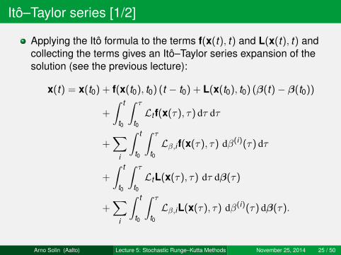
Applying the Itô formula to the terms f(x(t), t) and L(x(t), t) andcollecting the terms gives an Itô–Taylor series expansion of thesolution (see the previous lecture):
x(t) = x(t0) + f(x(t0), t0) (t − t0) + L(x(t0), t0) (β(t)− β(t0))
+
∫ t
t0
∫ τ
t0Lt f(x(τ), τ) dτ dτ
+∑
i
∫ t
t0
∫ τ
t0Lβ,i f(x(τ), τ) dβ(i)(τ) dτ
+
∫ t
t0
∫ τ
t0LtL(x(τ), τ) dτ dβ(τ)
+∑
i
∫ t
t0
∫ τ
t0Lβ,iL(x(τ), τ) dβ(i)(τ) dβ(τ).
Arno Solin (Aalto) Lecture 5: Stochastic Runge–Kutta Methods November 25, 2014 25 / 50
Itô–Taylor series [1/3]
The first row in the equation is just the Euler–Maruyama scheme.Similarly as we did in for the ordinary RK methods, we canconsider truncated series expansions of various degrees for eachof these terms.The extra terms involving the iterated and cross-term Itô integralscomplicate the formulation.To present a family of actual numerical methods, we consider thefollowing family of strong order 1.0 methods due to AndreasRößler...
Arno Solin (Aalto) Lecture 5: Stochastic Runge–Kutta Methods November 25, 2014 26 / 50
A class of SRK methods of strong order 1.0 [1/3]
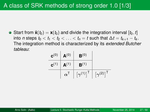
Start from x(t0) = x(t0) and divide the integration interval [t0, t ]into n steps t0 < t1 < t2 < . . . < tn = t such that ∆t = tk+1 − tk .The integration method is characterized by its extended Butchertableau:
c(0) A(0) B(0)
c(1) A(1) B(1)
αT [γ(1)]T [
γ(2)]T
Arno Solin (Aalto) Lecture 5: Stochastic Runge–Kutta Methods November 25, 2014 27 / 50

A class of SRK methods of strong order 1.0 [2/3]
On each step k approximate the solution trajectory as follows:
x(tk+1) = x(tk ) +s∑
i=1
αi f(x(0)i , tk + c(0)
i ∆t) ∆t
+s∑
i=1
m∑n=1
(γ(1)i ∆β
(n)k + γ
(2)i
√∆t) Ln(x(n)
i , tk + c(1)i ∆t)
Arno Solin (Aalto) Lecture 5: Stochastic Runge–Kutta Methods November 25, 2014 28 / 50
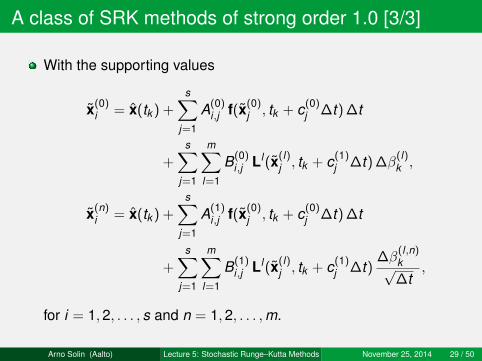
A class of SRK methods of strong order 1.0 [3/3]
With the supporting values
x(0)i = x(tk ) +
s∑j=1
A(0)i,j f(x(0)
j , tk + c(0)j ∆t) ∆t
+s∑
j=1
m∑l=1
B(0)i,j Ll(x(l)
j , tk + c(1)j ∆t) ∆β
(l)k ,
x(n)i = x(tk ) +
s∑j=1
A(1)i,j f(x(0)
j , tk + c(0)j ∆t) ∆t
+s∑
j=1
m∑l=1
B(1)i,j Ll(x(l)
j , tk + c(1)j ∆t)
∆β(l,n)k√∆t
,
for i = 1,2, . . . , s and n = 1,2, . . . ,m.
Arno Solin (Aalto) Lecture 5: Stochastic Runge–Kutta Methods November 25, 2014 29 / 50

The increments [1/2]
The increments in the algorithm are given by the Itô integrals:
∆β(i)k =
∫ tk+1
tkdβ(i)(τ) and
∆β(i,j)k =
∫ tk+1
tk
∫ τ2
tkdβ(i)(τ1) dβ(j)(τ2),
The increments ∆β(i)k are independent normally distributed
random variables∆β
(i)k ∼ N(0,∆t).
Arno Solin (Aalto) Lecture 5: Stochastic Runge–Kutta Methods November 25, 2014 30 / 50
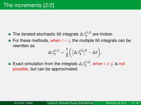
The increments [2/2]
The iterated stochastic Itô integrals ∆β(i,j)k are trickier.
For these methods, when i = j , the multiple Itô integrals can berewritten as
∆β(i,i)k =
12
([∆β
(i)k
]2 −∆t),
Exact simulation from the integrals ∆β(i,j)k , when i 6= j , is not
possible, but can be approximated.
Arno Solin (Aalto) Lecture 5: Stochastic Runge–Kutta Methods November 25, 2014 31 / 50

Example: Euler–Maruyama
Example (Euler–Maruyama Butcher tableau)The Euler–Maruyama method has the extended Butcher tableau:
0 0 00 0 0
1 1 0
and as we recall from the previous chapter, it is of strong order 0.5.
Arno Solin (Aalto) Lecture 5: Stochastic Runge–Kutta Methods November 25, 2014 32 / 50

Example: A strong order 1.0 method
Example (Strong order 1.0 SRK due to Rößler)Consider a stochastic Runge–Kutta method with the followingextended Butcher tableau:
01 1 00 0 0 0 001 1 11 1 0 −1 0
12
12 0 1 0 0 0 1
2 −12
The (rather lengthy) algorithm is written out in the lecture notes(Alg. 6.3).
Arno Solin (Aalto) Lecture 5: Stochastic Runge–Kutta Methods November 25, 2014 33 / 50

Higher-order methods
Higher-order methods by considering more terms in the Itô–Taylorexpansion.Not very practical in general (heavy and complicated).For models with some special structure this might still be feasible:
One-dimensional models.Additive noise models.Diagonal noise models.Models with commutative noise.
Arno Solin (Aalto) Lecture 5: Stochastic Runge–Kutta Methods November 25, 2014 34 / 50

Example: Duffing van der Pol oscillator [1/4]
Consider a simplified version of a Duffing van der Pol oscillator
x + x − (α− x2) x = x w(t), α ≥ 0,
driven by multiplicative white noise w(t) with spectral density q.The corresponding two-dimensional, x(t) = (x , x), Itô stochasticdifferential equation is(
dx1dx2
)=
(x2
(x1(α− x21 )− x2
)dt +
(0x1
)dβ,
where β(t) is a one-dimensional Brownian motion.Consider different initializations with q = 0 and q = 0.52. Use thesame realizations of noise for each initialization. Use α = 1 and∆t = 2−5.
Arno Solin (Aalto) Lecture 5: Stochastic Runge–Kutta Methods November 25, 2014 35 / 50

Example: Duffing van der Pol oscillator [2/4]
�4 �2 2 4
�4
�2
2
4
6
8
x1
x2
Arno Solin (Aalto) Lecture 5: Stochastic Runge–Kutta Methods November 25, 2014 36 / 50
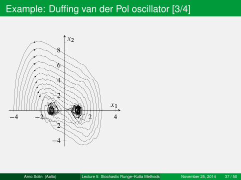
Example: Duffing van der Pol oscillator [3/4]
�4 �2 2 4
�4
�2
2
4
6
8
x1
x2
Arno Solin (Aalto) Lecture 5: Stochastic Runge–Kutta Methods November 25, 2014 37 / 50
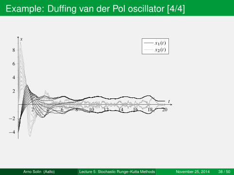
Example: Duffing van der Pol oscillator [4/4]
2 4 6 8 10 12 14 16 18 20
�4
�2
2
4
6
8
t
xx1.t/
x2.t/
Arno Solin (Aalto) Lecture 5: Stochastic Runge–Kutta Methods November 25, 2014 38 / 50
Weak stochastic Runge–Kutta methods
It is possible to form weak approximations to SDEs, where theinterest is not in the solution trajectories, but the distribution ofthem.We can replace weak Itô–Taylor approximations by Runge–Kuttastyle approximations which avoid the use of derivatives of the driftand diffusion coefficients.The reasoning behind the methods is very much the same as forstrong SRK methods.Here we consider a rather general class of weak order 2.0methods by Rößler:
Arno Solin (Aalto) Lecture 5: Stochastic Runge–Kutta Methods November 25, 2014 40 / 50
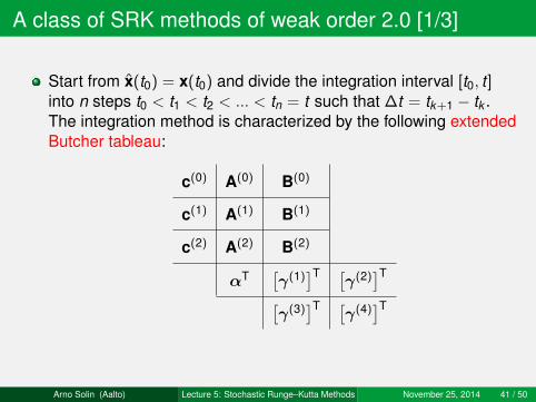
A class of SRK methods of weak order 2.0 [1/3]
Start from x(t0) = x(t0) and divide the integration interval [t0, t ]into n steps t0 < t1 < t2 < ... < tn = t such that ∆t = tk+1 − tk .The integration method is characterized by the following extendedButcher tableau:
c(0) A(0) B(0)
c(1) A(1) B(1)
c(2) A(2) B(2)
αT [γ(1)]T [
γ(2)]T[γ(3)]T [
γ(4)]T
Arno Solin (Aalto) Lecture 5: Stochastic Runge–Kutta Methods November 25, 2014 41 / 50

A class of SRK methods of weak order 2.0 [2/3]
On each step k approximate the solution by the following:
x(tk+1) = x(tk ) +s∑
i=1
αi f(x(0)i , tk + c(0)
i ∆t) ∆t
+s∑
i=1
m∑n=1
γ(1)i Ln(x(n)
i , tk + c(1)i ∆t) ∆β
(n)k
+s∑
i=1
m∑n=1
γ(2)i Ln(x(n)
i , tk + c(1)i ∆t)
∆β(n,n)k√∆t
+s∑
i=1
m∑n=1
γ(3)i Ln(x(n)
i , tk + c(2)i ∆t) ∆β
(n)k
+s∑
i=1
m∑n=1
γ(4)i Ln(x(n)
i , tk + c(2)i ∆t)
√∆t ,
Arno Solin (Aalto) Lecture 5: Stochastic Runge–Kutta Methods November 25, 2014 42 / 50
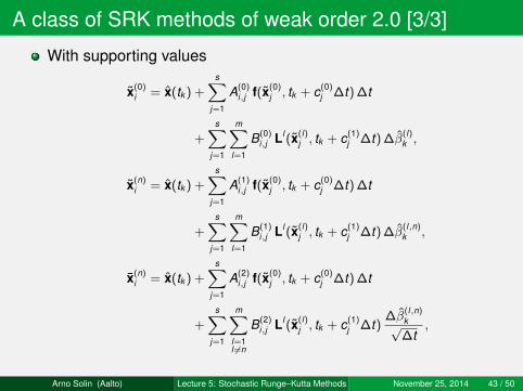
A class of SRK methods of weak order 2.0 [3/3]
With supporting values
x(0)i = x(tk ) +
s∑j=1
A(0)i,j f(x(0)
j , tk + c(0)j ∆t) ∆t
+s∑
j=1
m∑l=1
B(0)i,j Ll (x(l)
j , tk + c(1)j ∆t) ∆β
(l)k ,
x(n)i = x(tk ) +
s∑j=1
A(1)i,j f(x(0)
j , tk + c(0)j ∆t) ∆t
+s∑
j=1
m∑l=1
B(1)i,j Ll (x(l)
j , tk + c(1)j ∆t) ∆β
(l,n)k ,
x(n)i = x(tk ) +
s∑j=1
A(2)i,j f(x(0)
j , tk + c(0)j ∆t) ∆t
+s∑
j=1
m∑l=1l 6=n
B(2)i,j Ll (x(l)
j , tk + c(1)j ∆t)
∆β(l,n)k√∆t
,
Arno Solin (Aalto) Lecture 5: Stochastic Runge–Kutta Methods November 25, 2014 43 / 50

The increments [1/2]
Again, the increments are given by the double Itô integrals.In the weak schemes we can use the following approximations:
∆β(i,j)k =
12
(∆β
(i)k ∆β
(j)k −
√∆t ζ(i)k
), if i < j ,
12
(∆β
(i)k ∆β
(j)k +
√∆t ζ(j)k
), if i > j ,
12
([∆β
(i)k ]2 −∆t
), if i = j .
Here only 2m − 1 independent random variables are needed.No problems with the cross-term integrals any more.
Arno Solin (Aalto) Lecture 5: Stochastic Runge–Kutta Methods November 25, 2014 44 / 50

The increments [2/2]
For example, we can choose ∆β(i)k such that they are independent
three-point distributed random variables:
P(∆β
(i)k = ±
√3 ∆t
)=
16
and P(∆β
(i)k = 0
)=
23,
The supporting variables ζ(i)k such that they are independenttwo-point distributed random variables.
P(ζ(i)k = ±
√∆t)
=12.
Arno Solin (Aalto) Lecture 5: Stochastic Runge–Kutta Methods November 25, 2014 45 / 50
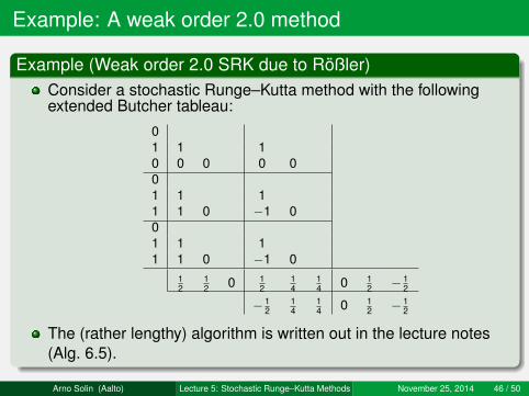
Example: A weak order 2.0 method
Example (Weak order 2.0 SRK due to Rößler)Consider a stochastic Runge–Kutta method with the followingextended Butcher tableau:
01 1 10 0 0 0 001 1 11 1 0 −1 001 1 11 1 0 −1 0
12
12 0 1
214
14 0 1
2 − 12
− 12
14
14 0 1
2 − 12
The (rather lengthy) algorithm is written out in the lecture notes(Alg. 6.5).
Arno Solin (Aalto) Lecture 5: Stochastic Runge–Kutta Methods November 25, 2014 46 / 50
Example: Weak SRK for Duffing van der Pol [1/2]
We are interested in characterizing the solution at t = 20 for theinitial condition of x(0) = (−3,0).We use the stochastic Runge–Kutta method of weak order 2.0.Discretization interval: ∆t = 2−4.We show the results as a histogram of x1(20) with 10,000samples.With a ∆t this large, the Euler–Maruyama method does notprovide plausible results.
Arno Solin (Aalto) Lecture 5: Stochastic Runge–Kutta Methods November 25, 2014 47 / 50

Example: Weak SRK for Duffing van der Pol [2/2]
�2 �1:5 �1 �0:5 0 0:5 1 1:5 2x1
Arno Solin (Aalto) Lecture 5: Stochastic Runge–Kutta Methods November 25, 2014 48 / 50

Summary
Stochastic Runge–Kutta methods are derivative-free methods forsolving SDEs.They cannot be derived as simple extensions to ordinaryRunge–Kutta methods.You cannot get rid of the iterated Itô integral.The complexity of the methods grows with the approximationorder.Higher order schemes can be practical for models with somespecial structure (scalar, additive, commutative, etc.).The choice between a weak and strong scheme depends on yourapplication.
Arno Solin (Aalto) Lecture 5: Stochastic Runge–Kutta Methods November 25, 2014 50 / 50