Lecture 5: Robot dynamics and simulation - Stanford University · 2019-01-23 · Lecture 5: Robot...

ME 328: Medical Robotics Winter 2019

Lecture 5:Robot dynamics and simulation

Allison OkamuraStanford University

Robot dynamics

equations of motion

describe the relationship between forces/torques and motion (in joint space or workspace variables)

two possible goals:

1. Given motion variables (e.g. or ), what joint torques ( ) or end-effector forces ( ) would have been the cause? (this is inverse dynamics)

~✓, ~✓, ~✓ ~x, ~x, ~x~⌧ ~f

2. Given joint torques ( ) or end-effector forces ( ), what motions (e.g. or ) would result? (this is forward dynamics)

~✓, ~✓, ~✓ ~x, ~x, ~x~⌧

~f

developing equations of motion using Lagrange’s equation

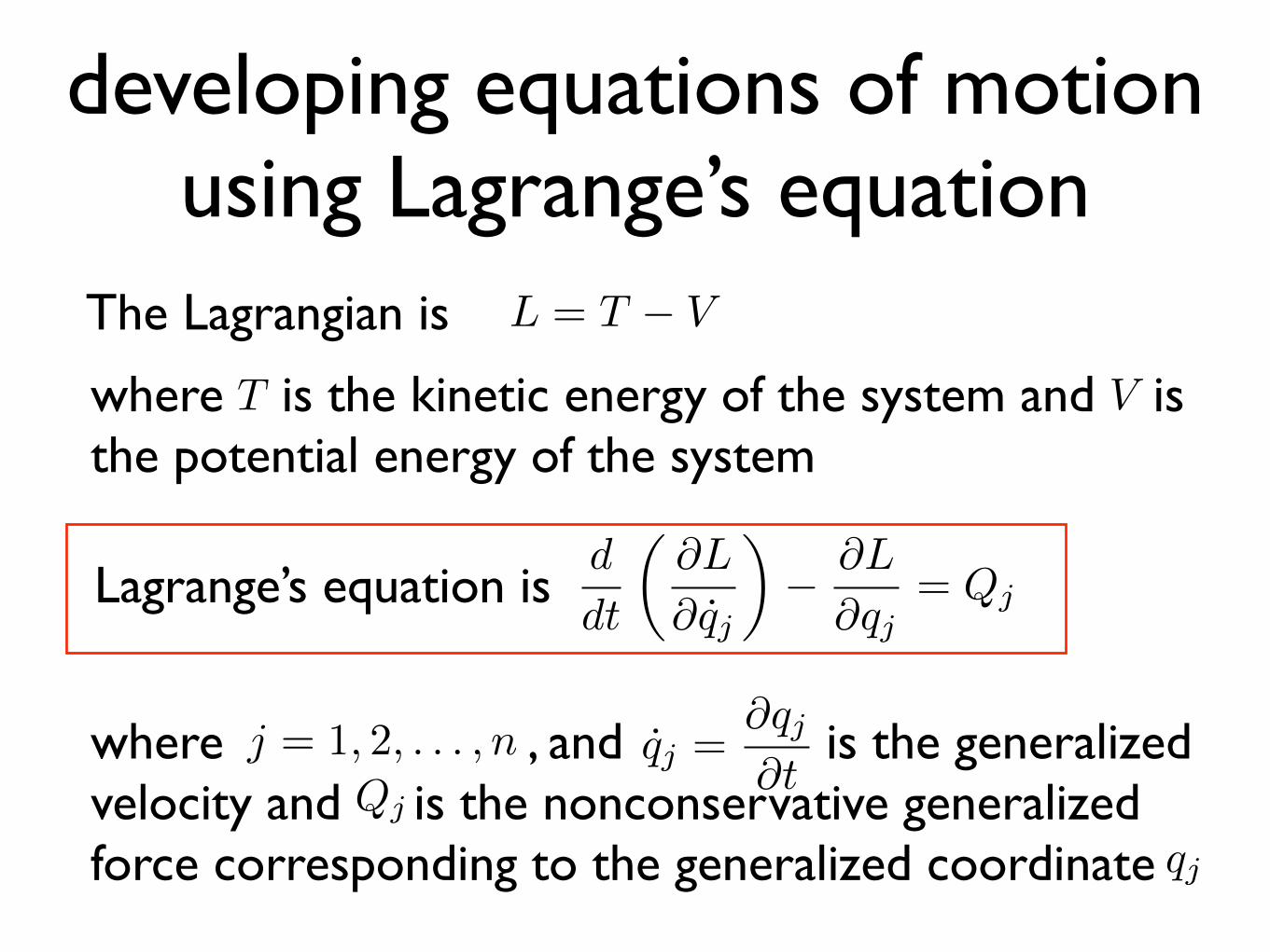
The Lagrangian is L = T � V

where is the kinetic energy of the system and is the potential energy of the system

T V

Lagrange’s equation isd

dt

✓@L

@qj

◆� @L

@qj= Qj

where , and is the generalized velocity and is the nonconservative generalized force corresponding to the generalized coordinate

j = 1, 2, . . . , n qj =@qj@tQj

qj

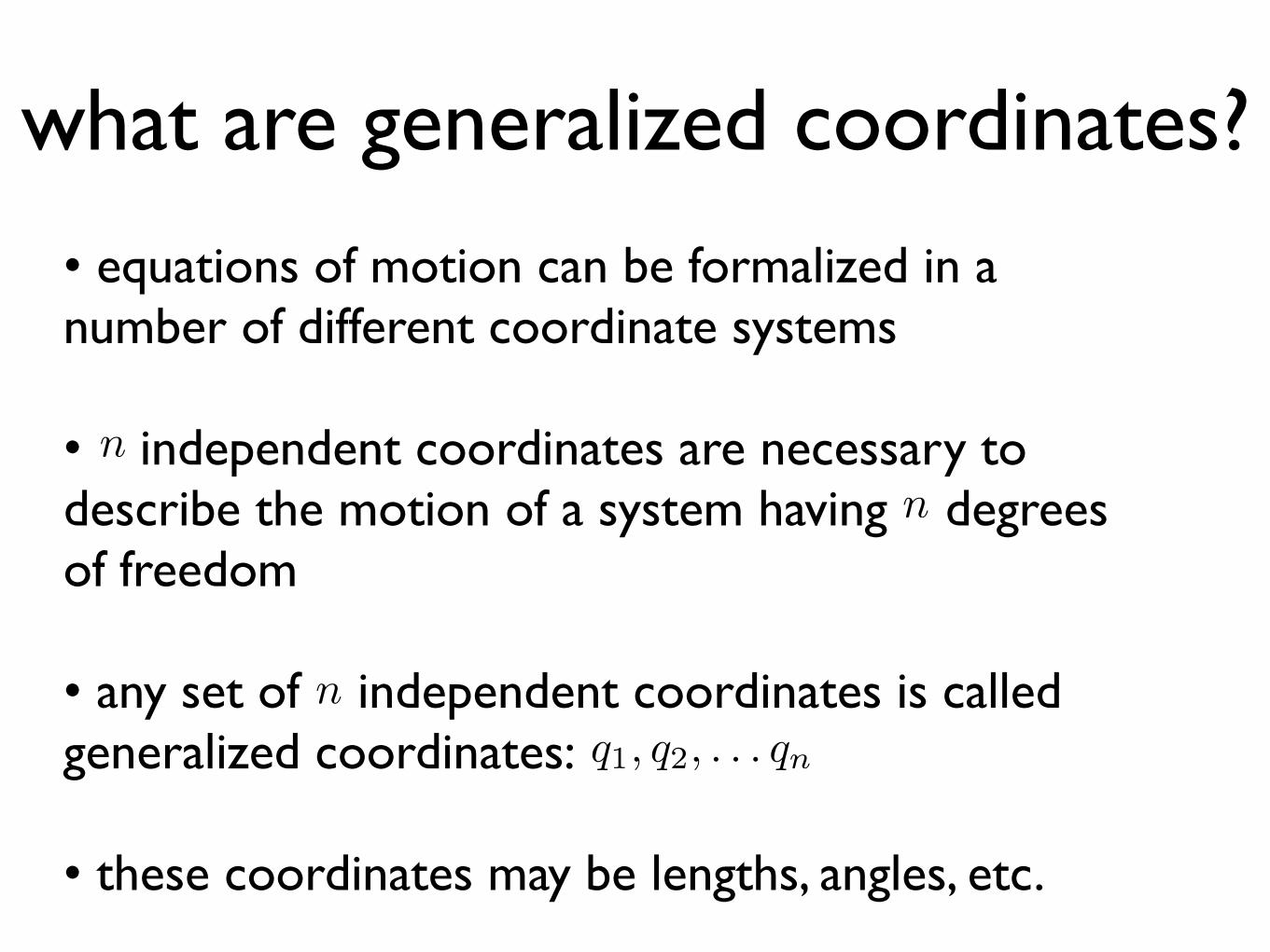
what are generalized coordinates?

• equations of motion can be formalized in a number of different coordinate systems

• independent coordinates are necessary to describe the motion of a system having degrees of freedom

• any set of independent coordinates is called generalized coordinates:

• these coordinates may be lengths, angles, etc.

n

n

nq1, q2, . . . qn

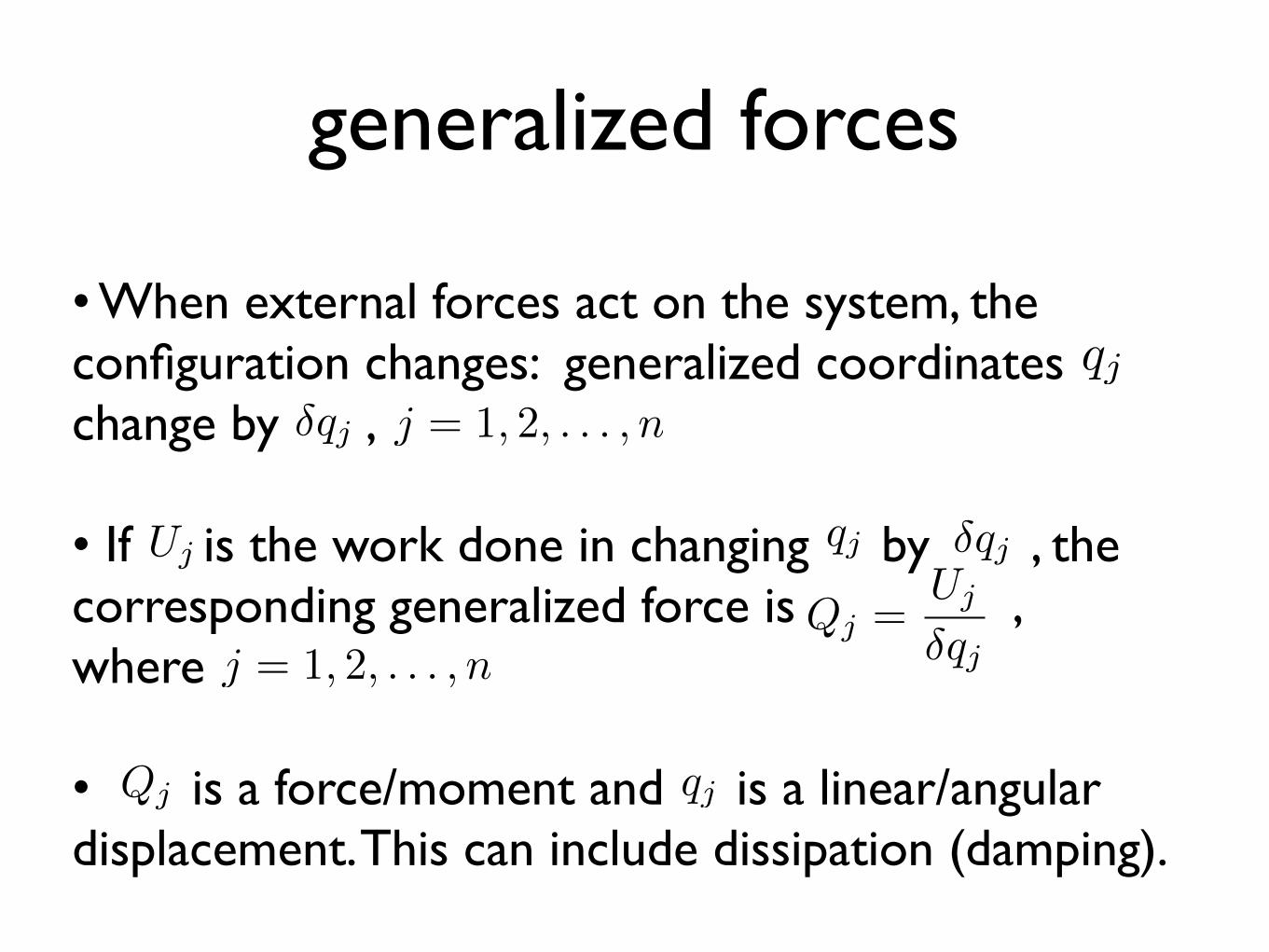
generalized forces

• When external forces act on the system, the configuration changes: generalized coordinates change by ,

• If is the work done in changing by , the corresponding generalized force is ,where

• is a force/moment and is a linear/angular displacement. This can include dissipation (damping).

qj

�qj

j = 1, 2, . . . , n

Ujqj

�qj

Qj =Uj

�qjj = 1, 2, . . . , n

qjQj

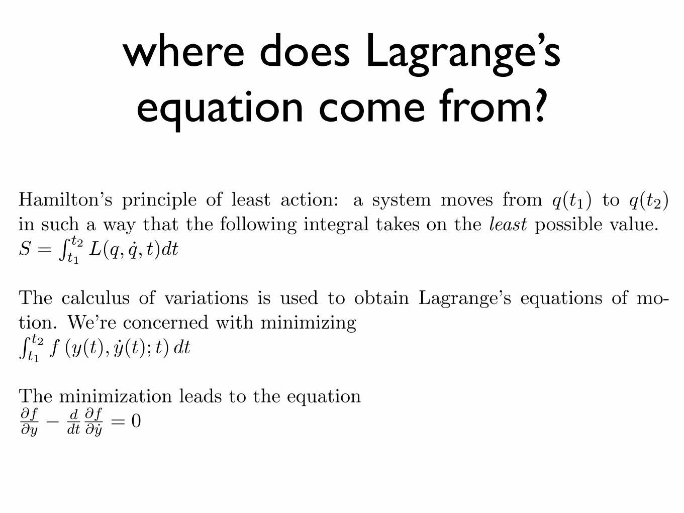
where does Lagrange’s equation come from?

ddt(

@L@qj

)� @L@qj

= Qj , where j = 1, 2, . . . , n

where qj =@qj@t is the generalized velocity and Qj is the nonconservative

generalized force corresponding to the generalized coordinate qj .

Where does it come from?

Hamilton’s principle of least action: a system moves from q(t1) to q(t2)in such a way that the following integral takes on the least possible value.

S =R t2t1

L(q, q, t)dt

The calculus of variations is used to obtain Lagrange’s equations of mo-

tion. We’re concerned with minimizingR t2t1

f (y(t), y(t); t) dt

The minimization leads to the equation@f@y � d

dt@f@y = 0

If there is more than one set of variables in the functional f (e.g. yi and yi)then you get one equation for each set.

To use for coupled systems, we need potential and kinetic energy expressions

in matrix form.

Define:

xi, displacement of mass mi

Fi, force applied in the direction of xi at mass mi

3

using Lagrange’s equation to derive equations of motion

This can be rewritten in matrix form:

T =12 x

TM x

where:

x =

2

6664

x1(t)x2(t)...

xn(t)

3

7775

M = diag(m1,m2, . . . ,mn)

In general, the mass matrix M might not be diagonal, for example if we

use a di↵erent set of generalized coordinates, such as the relative displace-

ments of the masses, rather than the absolute (ground-referenced) displace-

ment.

We can also use generalized coordinates:

V =12q

TKqK ! generalized sti↵ness matrix

T =12 q

TM qM ! generalized mass matrix

Note: In general, M need not be diagonal

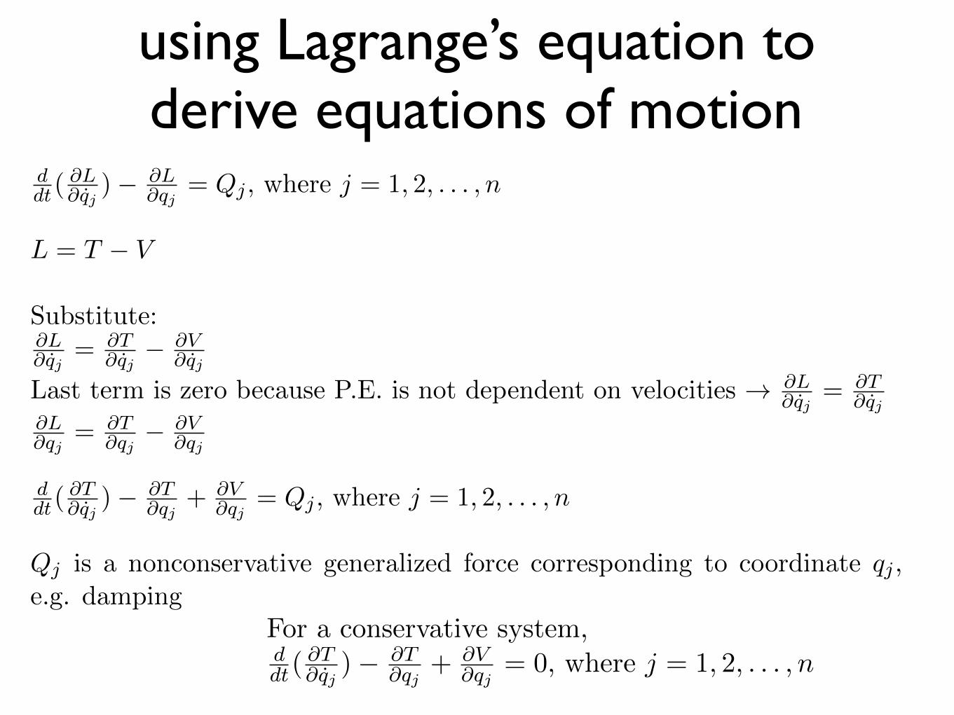
Using Lagrange’s Equation to derive Equations of Motion

ddt(

@L@qj

)� @L@qj

= Qj , where j = 1, 2, . . . , n

L = T � V

Substitute:@L@qj

=@T@qj

� @V@qj

Last term is zero because P.E. is not dependent on velocities ! @L@qj

=@T@qj

@L@qj

=@T@qj

� @V@qj

ddt(

@T@qj

)� @T@qj

+@V@qj

= Qj , where j = 1, 2, . . . , n

Qj is a nonconservative generalized force corresponding to coordinate qj ,e.g. damping

5

For a conservative system,ddt(

@T@qj

)� @T@qj

+@V@qj

= 0, where j = 1, 2, . . . , n

Example: Torsional System

Let q1 = ✓1, q2 = ✓2, q3 = ✓3

Kinetic energy:

T =12J1✓

21 +

12J2✓

22 +

12J3✓

23

Potential energy:

V =12k1✓

21 +

12k2(✓2 � ✓1)2 +

12k3(✓3 � ✓2)2

External moments are M1, M2, M3

Generalized force:

If Fxk, Fyk, Fzk are the external forces acting on the kth mass of the system

in the x, y, z directions:

Qj =P

k(Fxk@xk@qj

+ Fyk@yk@qj

+ Fzk@zk@qj

)

Where xk, yk, zk are the displacements of the kth mass in the x, y, z direc-

tions.

For a torsional system F is replaced by M , moment.

Qj =P3

k=1Mk@✓k@qj

=P3

k=1Mk@✓k@✓j

Q1 = M1@✓1@✓1

+M2@✓2@✓1

+M3@✓3@✓1

= M1

Q2 = M1@✓1@✓2

+M2@✓2@✓2

+M3@✓3@✓2

= M2

6

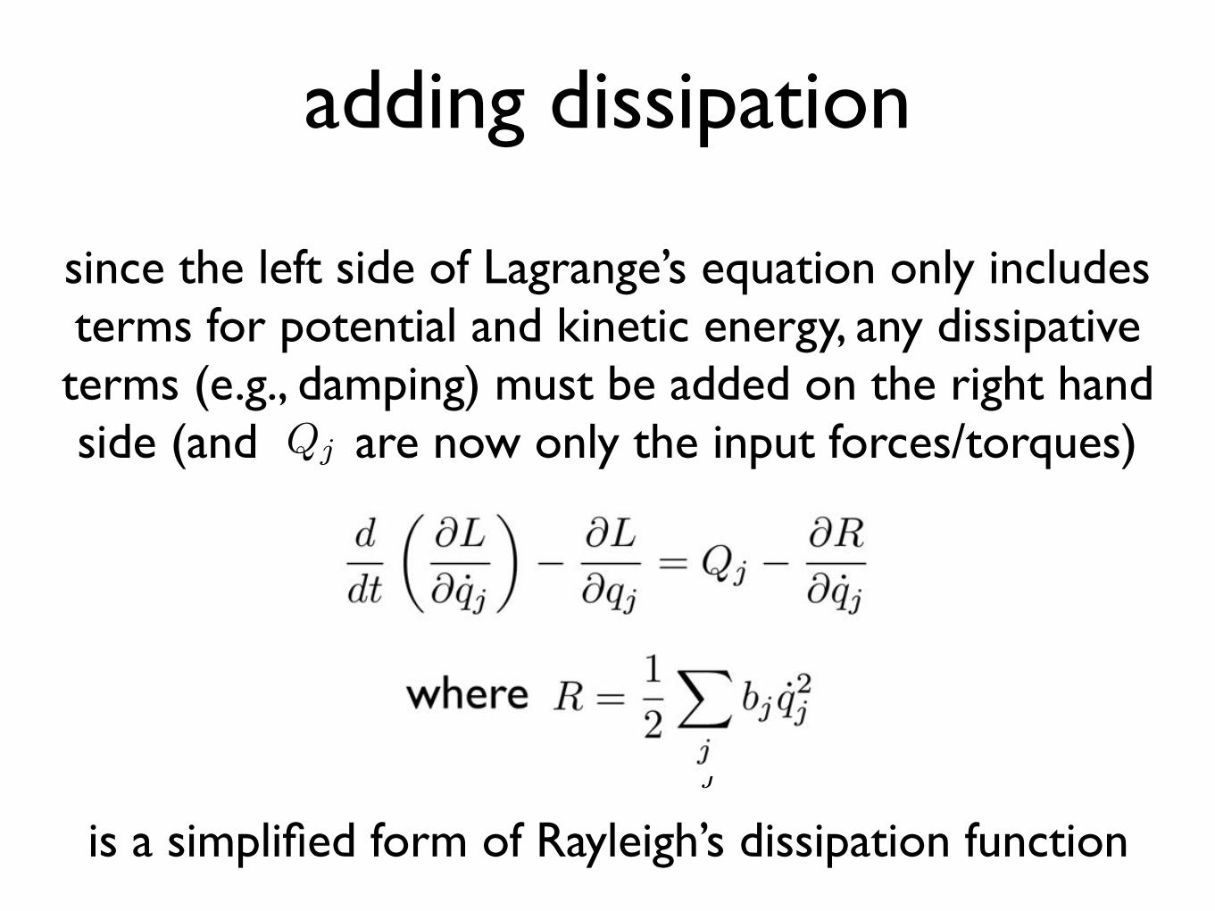
adding dissipation

since the left side of Lagrange’s equation only includes terms for potential and kinetic energy, any dissipative terms (e.g., damping) must be added on the right hand side (and are now only the input forces/torques)Qj

d

dt

✓@L

@qj

◆� @L

@qj= Qj �

@R

@qj

R =1

2

X

j

bj q2j

is a simplified form of Rayleigh’s dissipation function

example: double pendulum(review on your own)

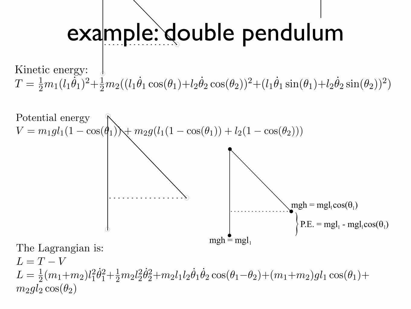
example: double pendulum

Double Pendulum Example

Velocity of m1: v1 = l1✓1Velocity of m2: v2 = (v22x + v22y)

12

v2x = l1✓1 cos(✓1) + l2✓2 cos(✓2)v2y = l1✓1 sin(✓1) + l2✓2 sin(✓2)

Kinetic energy:

T =12m1(l1✓1)2+

12m2((l1✓1 cos(✓1)+l2✓2 cos(✓2))2+(l1✓1 sin(✓1)+l2✓2 sin(✓2))2)

Potential energy

V = m1gl1(1� cos(✓1)) +m2g(l1(1� cos(✓1)) + l2(1� cos(✓2)))

3



12


Kinetic energy:

T =12m1(l1✓1)2+


Potential energy


3



12


Kinetic energy:

T =12m1(l1✓1)2+


Potential energy


3

The Lagrangian is:

L = T � VL =

12(m1+m2)l21✓

21+

12m2l22✓

22+m2l1l2✓1✓2 cos(✓1�✓2)+(m1+m2)gl1 cos(✓1)+

m2gl2 cos(✓2)

For ✓1:@L@✓1

= m1l21✓1 +m2l21✓1 +m2l1l2✓2 cos(✓1 � ✓2)

ddt

⇣@L@✓1

⌘= (m1+m2)l21✓1+m2l1l2✓2 cos(✓1�✓2)�m2l1l2✓2 sin(✓1�✓2)(✓1�✓2)

@L@✓1

= �l1g(m1 +m2) sin(✓1)�m2l1l2✓1✓2 sin(✓1 � ✓2)

Thus, the di↵erential equation for ✓1 becomes:

(m1 + m2)l21✓1 + m2l1l2✓2 cos(✓1 � ✓2) + m2l1l2✓22 sin(✓1 � ✓2) + l1g(m1 +

m2) sin(✓1) = 0

Divide through by l1 and this simplifies to:

(m1+m2)l1✓1+m2l2✓2 cos(✓1�✓2)+m2l2✓22 sin(✓1�✓2)+g(m1+m2) sin(✓1) =0

Similarly, for ✓2:@L@✓2

= m2l22✓2 +m2l1l2✓1 cos(✓1 � ✓2)

ddt

⇣@L@✓2

⌘= m2l2✓2 +m2l1l2✓1 cos(✓1 � ✓2)�m2l1l2✓1 sin(✓1 � ✓2)(✓1 � ✓2)

@L@✓2

= m2l1l2✓1✓2 sin(✓1 � ✓2)� l2m2g sin ✓2


m2l22✓2 +m2l1l2✓1 cos(✓1 � ✓2)�m2l1l2✓21 sin(✓1 � ✓2) + l2m2g sin ✓2 = 0


m2l2✓2 +m2l1✓1 cos(✓1 � ✓2)�m2l1✓21 sin(✓1 � ✓2) +m2g sin ✓2 = 0

So, we have developed a very complicated set of coupled equations of motion

from a very simple system!

For the initial conditions ✓1 =⇡2 and ✓2 = ⇡, you get the response be-

low. If you perturbed these initial conditions slightly, you would get a verydi↵erent response. This is evidence of a chaotic system. If you linearized

the equations or added damping, you would get a much more predictable

4

example: double pendulumThe Lagrangian is:

L = T � VL =

12(m1+m2)l21✓

21+

12m2l22✓

22+m2l1l2✓1✓2 cos(✓1�✓2)+(m1+m2)gl1 cos(✓1)+

m2gl2 cos(✓2)

For ✓1:@L@✓1

= m1l21✓1 +m2l21✓1 +m2l1l2✓2 cos(✓1 � ✓2)

ddt

⇣@L@✓1


@L@✓1

= �l1g(m1 +m2) sin(✓1)�m2l1l2✓1✓2 sin(✓1 � ✓2)



m2) sin(✓1) = 0




= m2l22✓2 +m2l1l2✓1 cos(✓1 � ✓2)

ddt

⇣@L@✓2

⌘= m2l2✓2 +m2l1l2✓1 cos(✓1 � ✓2)�m2l1l2✓1 sin(✓1 � ✓2)(✓1 � ✓2)

@L@✓2

= m2l1l2✓1✓2 sin(✓1 � ✓2)� l2m2g sin ✓2










4

example: double pendulum

The Lagrangian is:

L = T � VL =

12(m1+m2)l21✓

21+

12m2l22✓

22+m2l1l2✓1✓2 cos(✓1�✓2)+(m1+m2)gl1 cos(✓1)+

m2gl2 cos(✓2)

For ✓1:@L@✓1

= m1l21✓1 +m2l21✓1 +m2l1l2✓2 cos(✓1 � ✓2)

ddt

⇣@L@✓1


@L@✓1

= �l1g(m1 +m2) sin(✓1)�m2l1l2✓1✓2 sin(✓1 � ✓2)



m2) sin(✓1) = 0




= m2l22✓2 +m2l1l2✓1 cos(✓1 � ✓2)

ddt

⇣@L@✓2

⌘= m2l2✓2 +m2l1l2✓1 cos(✓1 � ✓2)�m2l1l2✓1 sin(✓1 � ✓2)(✓1 � ✓2)

@L@✓2

= m2l1l2✓1✓2 sin(✓1 � ✓2)� l2m2g sin ✓2










4

but robots are not point masses...links could be represented by solid cylinders

Iz =mr2

2

Ix = Iy =1

12m

�3r2 + h2

�

http://en.wikipedia.org/wiki/List_of_moments_of_inertia

moment of inertia tensor:

moments of inertia about center:

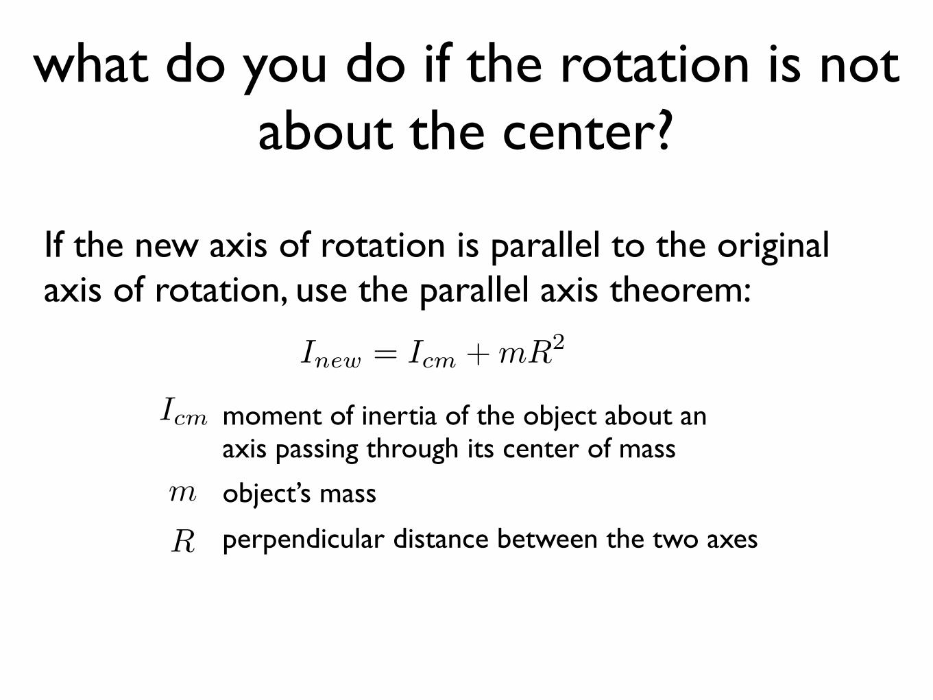
what do you do if the rotation is not about the center?

If the new axis of rotation is parallel to the original axis of rotation, use the parallel axis theorem:

Inew = Icm +mR2

Icm

m

R

moment of inertia of the object about an axis passing through its center of mass

object’s mass

perpendicular distance between the two axes

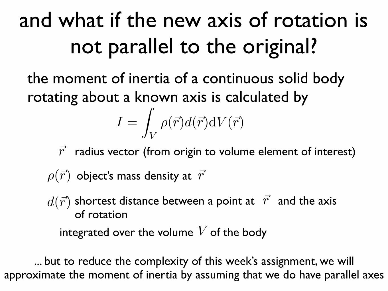
and what if the new axis of rotation is not parallel to the original?

the moment of inertia of a continuous solid body rotating about a known axis is calculated by

radius vector (from origin to volume element of interest)

object’s mass density at

shortest distance between a point at and the axis of rotation

I =

Z

V⇢(~r)d(~r)dV (~r)

⇢(~r)

~r

~r

d(~r) ~r

integrated over the volume of the body V

... but to reduce the complexity of this week’s assignment, we will approximate the moment of inertia by assuming that we do have parallel axes

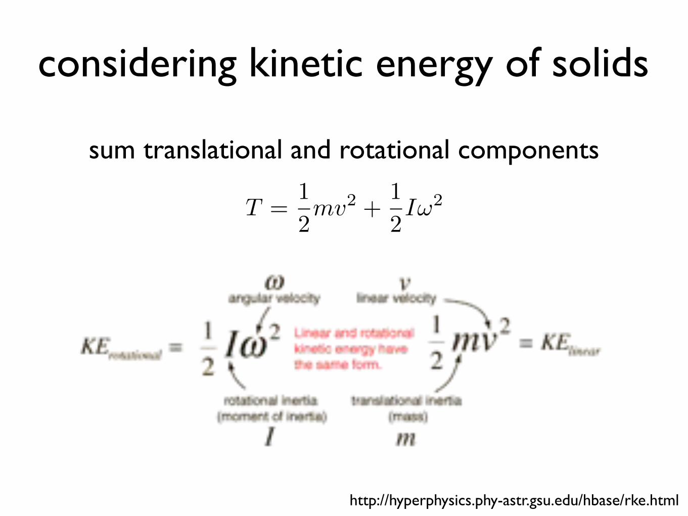
considering kinetic energy of solids

sum translational and rotational components

T =1

2mv2 +

1

2I!2

http://hyperphysics.phy-astr.gsu.edu/hbase/rke.html

for robot dynamics background

class: CS223A / ME320: Introduction to Robotics

dynamics and robotics textbooks such asJohn J. Craig

Introduction to Robotics: Mechanics and Control

… and many others

In Assignment 3, we will give you the dynamic equations, but it helps to understand where they come from!

questions

• how do you think an RCM robot compares to a typical serial chain manipulator in terms of its dynamics?

• does the da Vinci have haptic feedback? (and how do the system dynamics affect this capability?)

Dynamic simulation

controller on one end, system dynamics on the other

endpointforce/torque

desired force(in computer)

a controller computes the desired force

this force and externally applied loads result in robot motion

e.g. f = kp*(x-xd)

e.g., solve for x in f = mx+ bx

in Assignment 3,you will simulate the

effects of system dynamics

simulating equations of motion

goal: given an equation of motion and applied forces,what will the resulting robot motion be?

The dynamics equations we have are coupled, non-linear ODEs. They are hard (likely impossible) to solve analytically.

Instead, we solve them using numerical integration.

you can do a simple calculation yourself,i.e. integration using the trapezoidal rule, or use a handy

and more accurate/robust Matlab function(Simulink is also an option)

Numerical Solutions

In this course, we have primarily solved dynamic systems analytically, invoking Matlab to facilitateplotting and data manipulation. However, Matlab can also be a powerful tool for solving ordinarydi↵erential equations (ODEs) directly.

There are a series of native Matlab functions that solve ODEs given initial conditions. Di↵erentfunctions are appropriate for di↵erent problem types (“sti↵ness”, corresponding to large di↵erencesin scales) and and order of accuracy (low to high).

Solver Problem Type Order of Accuracy When to Use

ode45 Nonsti↵ Medium Most of the time. This should be the firstsolver you try.

ode23 Nonsti↵ Low For problems with crude error tolerances orfor solving moderately sti↵ problems.

ode113 Nonsti↵ Low to high For problems with stringent error tolerancesor for solving computationally intensive prob-lems.

ode15s Sti↵ Low to medium If ode45 is slow because the problem is sti↵.ode23s Sti↵ Low If using crude error tolerances to solve sti↵

systems and the mass matrix is constant.ode23t Moderately Sti↵ Low For moderately sti↵ problems if you need a

solution without numerical damping.ode23tb Sti↵ Low If using crude error tolerances to solve sti↵

systems.

ode45 is based on an explicit Runge-Kutta (4,5) formula, the Dormand-Prince pair. It is a one-stepsolver - in computing y(tn), it needs only the solution at the immediately preceding time point,y(tn-1). In general, ode45 is the best function to apply as a “first try” for most problems.

The basic syntax for these solvers is:[T,Y] = solver(odefun,tspan,y0)

where:solver is one of ode45, ode23, etc.odefun is a function handle that evaluates the right side of the di↵erential equationstspan is a vector specifying the interval of integration, [t0,tf]y0 is a vector of initial conditions

Example: First order system

Let’s say that we want to solve the function

y + 2y = 0

for the initial condition y(0) = 10.

3

Numerical Solutions










systems.






y + 2y = 0


3

Numerical Solutions










systems.






y + 2y = 0


3

Numerical Solutions










systems.






y + 2y = 0


3

First, you need to create a function of the form y = f(t, y):function ydot = my_function(t,y)

ydot = -2*y; % end of subprogram

And the code to apply initial condition and solve the system is:tspan = [0,5]; % time duration for calculation

y0 = 10; % initial condition

% Note that the equation of motion is in a

% subprogram named my_func

[t,y] = ode45(’my_func’,tspan,y0);

% plot the response

figure

plot(t,y)

title(’First Order Response’)

xlabel(’Time (s)’)

ylabel(’Position (m)’)

The resulting plot is shown below:

0 0.5 1 1.5 2 2.5 3 3.5 4 4.5 50

1

2

3

4

5

6

7

8

9

10First Order Response

Time (s)

Posit

ion

(m)

Example: Second order system

We will now look at the response of a second order system, an inverted pendulum with the followingequation of motion:

✓ � g

lsin(✓) = 0

4

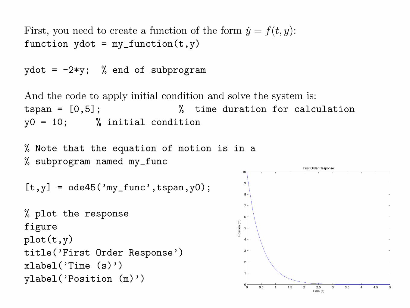
First, you need to create a function of the form y = f(t, y):function ydot = my_function(t,y)

ydot = -2*y; % end of subprogram

And the code to apply initial condition and solve the system is:tspan = [0,5]; % time duration for calculation

y0 = 10; % initial condition

% Note that the equation of motion is in a

% subprogram named my_func

[t,y] = ode45(’my_func’,tspan,y0);

% plot the response

figure

plot(t,y)

title(’First Order Response’)

xlabel(’Time (s)’)

ylabel(’Position (m)’)

The resulting plot is shown below:

0 0.5 1 1.5 2 2.5 3 3.5 4 4.5 50

1

2

3

4

5

6

7

8

9

10First Order Response

Time (s)

Posit

ion

(m)

Example: Second order system

We will now look at the response of a second order system, an inverted pendulum with the followingequation of motion:

✓ � g

lsin(✓) = 0

4

trajectory generation

reference: Chapter 7 of Introduction to Robotics by J. J. Craig (any edition)

discussion

why would you want to generate a trajectory?

would you want to do trajectory generation in Cartesian space or joint space?

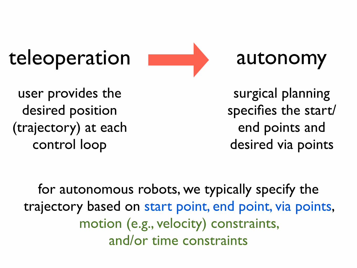
teleoperation autonomy

user provides the desired position

(trajectory) at each control loop

surgical planning specifies the start/

end points and desired via points

for autonomous robots, we typically specify the trajectory based on start point, end point, via points,

motion (e.g., velocity) constraints, and/or time constraints

discussion

what properties might you want in a trajectory?

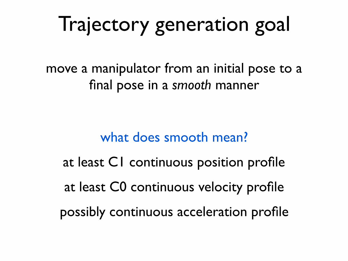
Trajectory generation goal

move a manipulator from an initial pose to a final pose in a smooth manner

what does smooth mean?

at least C1 continuous position profile

at least C0 continuous velocity profile

possibly continuous acceleration profile

point-to-point trajectory generation

consider the problem of moving a robot end-effector from its initial 3D pose to a final 3D pose

in a certain amount of time

robot graphic courtesy Fidel Hernandez

p(0) p(tf )p(t) =

2

4x(t)y(t)z(t)

3

5

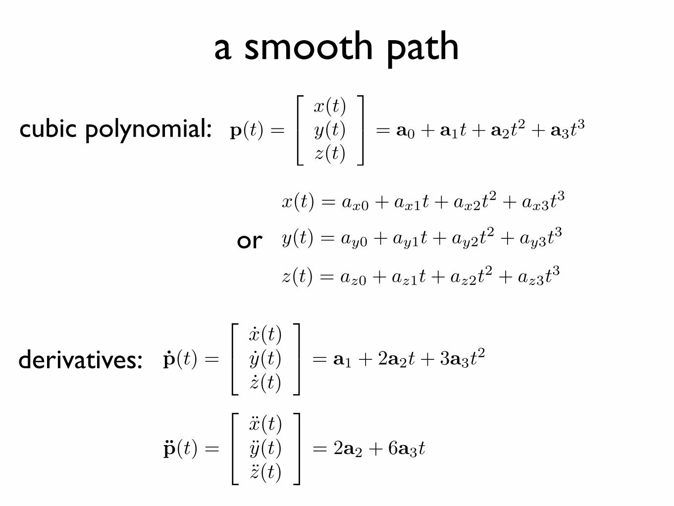
a smooth path

cubic polynomial: p(t) =

2

4x(t)y(t)z(t)

3

5 = a0 + a1t+ a2t2 + a3t3

or

x(t) = ax0 + ax1t+ ax2t2 + ax3t3

y(t) = ay0 + ay1t+ ay2t2 + ay3t3

z(t) = az0 + az1t+ az2t2 + az3t3

derivatives: p(t) =

2

4x(t)y(t)z(t)

3

5 = a1 + 2a2t+ 3a3t2

p(t) =

2

4x(t)y(t)z(t)

3

5 = 2a2 + 6a3t

constraintsposition and velocity at initial and final times:

with four equations and four unknowns, you can solve for the coefficients in terms of and

and the time

p(0) = p0

p(tf ) = pf

p(0) = 0p(tf ) = 0

a p0 pf

you can pick the time based on how quickly you want to move between to the two points, or based

on a maximum velocity constraint

tf

tf

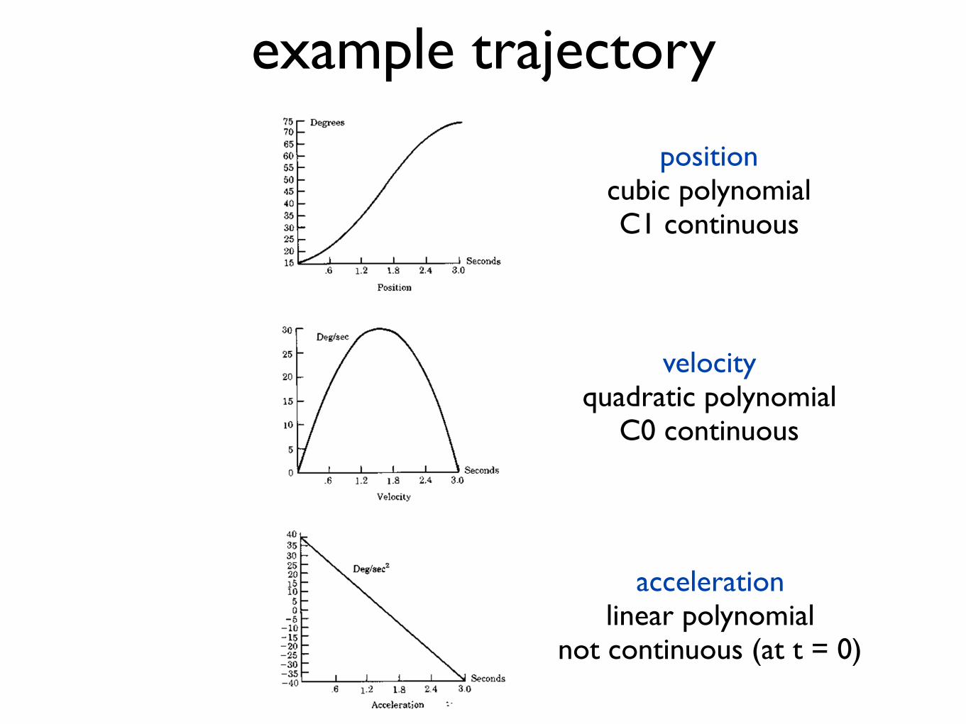
example trajectoryExample

Position

Acceleration

Velocity

A single-link robot with a rotary joint

• Must start and stop at rest

• Must start from θ0 = 15° and stop at θf = 75°• Must do so in tf = 3 seconds

344.4200.2000.15)( ttt −++=θ

233.1300.40)(.

ttt +=θ

tt 66.2600.40)(..

−=θ

positioncubic polynomialC1 continuous

velocityquadratic polynomial

C0 continuous

accelerationlinear polynomial

not continuous (at t = 0)

now what?

now that you have created a trajectory(i.e., you know the desired position

of the robot at each time step),you can control the robot to follow

this trajectory

previously, we generated this trajectoryusing the “master” of the teleoperator

discussion

why is a smooth trajectory important?why might you want a smoother trajectory?

how could you compute this?

what do the produced trajectories look like spatially? what if you design in joint space instead of Cartesian space?

how might via points be useful?how would you generate trajectories for them?

discussion

how would you compute based on a defined maximum velocity?

what kind of trajectory would you want for arobot that inserts a needle into solid tissue?

tf

bloodbot (Imperial College of London)

Overview

user input or trajectory

x(t)PD

controller plantxd(t)

gpd, similar to Assignment 2

dynamic model or physical robot

-+

x’(t) = f(x(t), gpd(x(t), xd(t)))

forces

the ODE we solve numerically

Assignment 3Problem 0: Commentary on seminar

Problem 1: Read papers, answer questions

Problem 2: Modeling and simulation of medical robot dynamics

Problem 3: Effects of dynamics on robot control

To be posted tomorrow, due Thursday, Jan. 31 at 4 pm

FRIDAY’S SEMINAR IS AT 8:30 am! (in 320-105)

Lecture 5: Robot dynamics and simulation - Stanford University · 2019-01-23 · Lecture 5: Robot...

Documents

Transcript of Lecture 5: Robot dynamics and simulation - Stanford University · 2019-01-23 · Lecture 5: Robot...