Lecture 5 - Computer Science - Western Universityolga/Courses/CS434a_541a/Lecture5.pdf · Prof....
36
CS434a/541a: Pattern Recognition Prof. Olga Veksler Lecture 5
Transcript of Lecture 5 - Computer Science - Western Universityolga/Courses/CS434a_541a/Lecture5.pdf · Prof....
CS434a/541a: Pattern RecognitionProf. Olga Veksler
Lecture 5
Today
� Introduction to parameter estimation� Two methods for parameter estimation
� Maximum Likelihood Estimation� Bayesian Estimation

Introducton� Bayesian Decision Theory in previous lectures
tells us how to design an optimal classifier if we knew:� P(ci) (priors)� P(x | ci) (class-conditional densities)
� Unfortunately, we rarely have this complete information!
� Suppose we know the shape of distribution, but not the parameters � Two types of parameter estimation
� Maximum Likelihood Estimation� Bayesian Estimation

ML and Bayesian Parameter Estimation
� Shape of probability distribution is known� Happens sometimes
� Labeled training data
a lot is known”easier”
little is known“harder”
salmon salmonsalmonbass
� Need to estimate parameters of probability distribution from the training data
Example
(((( ))))211,N σσσσµµµµ
(((( ))))222 ,N σσσσµµµµ
222
211 ,,, σσσσµµµµσσσσµµµµ
respected fish expert says salmon’s length has distribution and sea bass’s length has distribution
� Need to estimate parameters� Then design classifiers according to the bayesian decision theory

Independence Across Classes
� We have training data for each classsalmon salmon salmonsea bass sea bass sea bass
� When estimating parameters for one class, will only use the data collected for that class� reasonable assumption that data from class ci gives
no information about distribution of class cj
estimate parameters for distribution of salmon from
estimate parameters for distribution of bass from

Independence Across Classes
� For each class ci we have a proposed density pi(x| ci) with unknown parameters θ θ θ θ i which we need to estimate
� Since we assumed independence of data across the classes, estimation is an identical procedure for all classes
� To simplify notation, we drop sub-indexes and say that we need to estimate parameters θθθθ for density p(x) � the fact that we need to do so for each class on the
training data that came from that class is implied

� Bayesian Estimation� Parameters θθθθ are random variables having some
known a priori distribution (prior)
ML vs. Bayesian Parameter Estimation
� Maximum Likelihood� Parameters θθθθ are unknown but fixed (i.e. not
random variables)
� After parameters are estimated with either ML or Bayesian Estimation we use methods from Bayesian decision theory for classification
p(θθθθ)
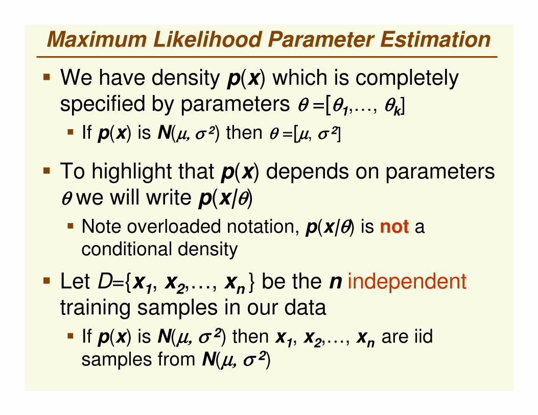
� We have density p(x) which is completely specified by parameters θθθθ =[θθθθ1,…, θθθθk]� If p(x) is N(µ, σ µ, σ µ, σ µ, σ 2) then θθθθ =[µµµµ, σ σ σ σ 2]
Maximum Likelihood Parameter Estimation
� Let D={x1, x2,…, xn } be the n independent training samples in our data� If p(x) is N(µ, σ µ, σ µ, σ µ, σ 2) then x1, x2,…, xn are iid
samples from N(µ, σ µ, σ µ, σ µ, σ 2)
� To highlight that p(x) depends on parameters θθθθ we will write p(x|θθθθ)� Note overloaded notation, p(x|θθθθ) is not a
conditional density

Maximum Likelihood Parameter Estimation� Consider the following function, which is
called likelihood of θθθθ with respect to the set of samples D
)(F)|x(p)|D(pnk
1kk θθθθθθθθθθθθ ======== ∏∏∏∏
====
====
� Note if D is fixed p(D|θθθθ) is not a density
� Maximum likelihood estimate (abbreviated MLE) of θθθθ is the value of θθθθ that maximizes the likelihood function p(D|θθθθ)
(((( )))))|D(pmaxargˆ θθθθθθθθθθθθ
====
Maximum Likelihood Estimation (MLE)
)|x(p)|D(pnk
1kk θθθθθθθθ ∏∏∏∏
====
====
====
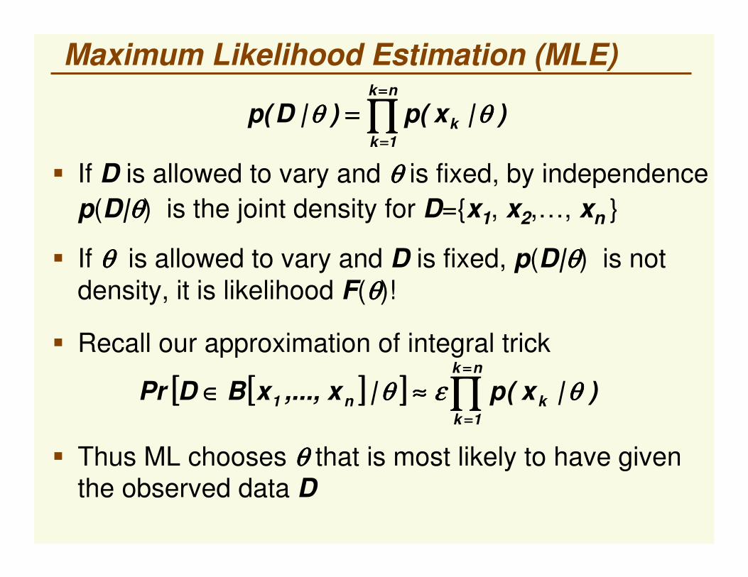
� If D is allowed to vary and θθθθ is fixed, by independence p(D|θθθθ) is the joint density for D={x1, x2,…, xn }
� If θθθθ is allowed to vary and D is fixed, p(D|θθθθ) is not density, it is likelihood F(θθθθ)!
� Recall our approximation of integral trick
[[[[ ]]]][[[[ ]]]] )|x(p|x,...,xBDPrnk
1kkn1 θθθθεεεεθθθθ ∏∏∏∏
====
====
≈≈≈≈∈∈∈∈
� Thus ML chooses θθθθ that is most likely to have given the observed data D

ML Parameter Estimation vs. ML Classifier
decide class ci which maximizes p(x|ci)
� Recall ML classifierfixeddata
choose θθθθ that maximizes p(D|θθθθ)
� Compare with ML parameter estimationfixeddata
� ML classifier and ML parameter estimation use the same principles applied to different problems

Maximum Likelihood Estimation (MLE)
� Instead of maximizing p(D|θθθθ), it is usually easier to minimize ln(p(D|θθθθ))
(((( ))))
(((( )))))|D(plnmaxarg
)|D(pmaxargˆ
θθθθ
θθθθθθθθ
θθθθ
θθθθ
====
========
� To simplify notation, ln(p(D|θθθθ))=l(θθθθ)
(((( )))) (((( ))))������������
����������������
����====������������
����������������
����======== ����∏∏∏∏====
====
====
n
1kk
nk
1kk |xplnmaxarg)|x(plnmaxarglmaxargˆ θθθθθθθθθθθθθθθθ
θθθθθθθθθθθθ
p(D|θθθθ)
ln(p(D|θθθθ))
� Since log is monotonic

2
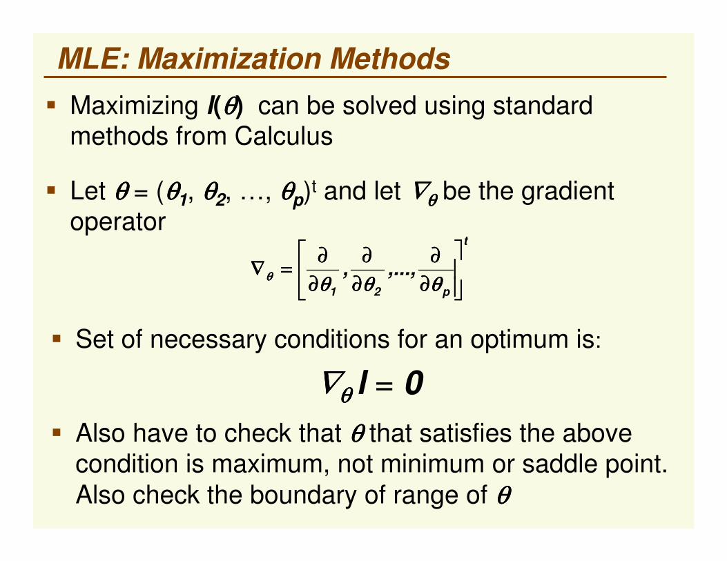
� Let θθθθ = (θθθθ1, θθθθ2, …, θθθθp)t and let ∇∇∇∇θθθθ be the gradient operator
t
p21
,...,,��������
������������
∂∂∂∂∂∂∂∂
∂∂∂∂∂∂∂∂
∂∂∂∂∂∂∂∂====∇∇∇∇
θθθθθθθθθθθθθθθθ
MLE: Maximization Methods� Maximizing l(θθθθ) can be solved using standard
methods from Calculus
� Set of necessary conditions for an optimum is:
∇∇∇∇θθθθ l = 0� Also have to check that θθθθ that satisfies the above
condition is maximum, not minimum or saddle point. Also check the boundary of range of θθθθ

� Let’s go through an example anyway
MLE Example: Gaussian with unknown µµµµ� Fortunately for us, all the ML estimates of any
densities we would care about have been computed
� Let p(x| µµµµ) be N(µµµµ,σ σ σ σ 2) that is σ σ σ σ 2 is known, but µµµµ is unknown and needs to be estimated, so θθθθ = µµµµ
(((( )))) (((( )))) ====������������
����������������
����======== ����====
n
1kk |xplnmaxarglmaxargˆ µµµµµµµµµµµµ
µµµµµµµµ
(((( ))))====
��������
����
����
��������
����
����
��������
����
����
��������
����
����������������
����������������
���� −−−−−−−−==== ����====
n
1k2
2k
2x
exp21
lnmaxargσσσσ
µµµµπσπσπσπσµµµµ
(((( ))))����
====������������
����������������
���� −−−−−−−−−−−−====n
1k2
2k
2x
2lnmaxargσσσσ
µµµµπσπσπσπσµµµµ

MLE Example: Gaussian with unknown µµµµ
� Thus the ML estimate of the mean is just the average value of the training data, very intuitive!� average of the training data would be our guess for
the mean even if we didn’t know about ML estimates
(((( ))))(((( )))) (((( ))))����
====������������
����������������
���� −−−−−−−−−−−−====n
1k2
2k
2x
2lnmaxarglmaxargσσσσ
µµµµπσπσπσπσµµµµµµµµµµµµ
(((( ))))(((( )))) (((( )))) 0x1
ldd n
1kk2 ====−−−−==== ����
====µµµµ
σσσσµµµµ
µµµµ���� 0nx
n
1kk ====−−−−����
====µµµµ
����====
====n
kkx
n 1
1µ̂µµµ
����
����

MLE for Gaussian with unknown µµµµ, σ σ σ σ 2222
� Similarly it can be shown that if p(x| µµµµ,ΣΣΣΣ) is N(µµµµ, ΣΣΣΣ), that is x is a multivariate gaussian with both mean and covariance matrix unknown, then
����====
====n
kkx
n 1
1µ̂µµµ (((( ))))(((( ))))����====
−−−−−−−−====n
1k
tkk ˆxˆx
n1ˆ µµµµµµµµΣΣΣΣ
� Similarly it can be shown that if p(x| µµµµ,σ σ σ σ 2222) is N(µµµµ, σ σ σ σ 2222), that is x both mean and variance are unknown, then again very intuitive result
����====
====n
kkx
n 1
1µ̂µµµ (((( ))))����====
−−−−====n
kkx
n 1
22 ˆ1
ˆ µµµµσσσσ

Today
� Finish Maximum Likelihood Estimation� Bayesian Parameter estimation� New Topic
� Non Parametric Density Estimation

� How good is a ML estimate ? � or actually any other estimate of a parameter?
How to Measure Performance of MLE?
� The natural measure of error would be θθθθθθθθ ˆ−−−−
θθθθ̂
� But is random, we cannot compute it before we carry out experiments
θθθθθθθθ ˆ−−−−
� We want to say something meaningful about our estimate as a function of θθθθ
� A way to solve this difficulty is to average the error, i.e. compute the mean absolute error
[[[[ ]]]] (((( ))))���� −−−−====−−−− n21n21 dx...dxdxx,...,x,xpˆˆE θθθθθθθθθθθθθθθθ

How to Measure Performance of MLE?s
(((( ))))[[[[ ]]]]2ˆE θθθθθθθθ −−−−
� It is usually much easier to compute an almost equivalent measure of performance, the mean squared error:
� Do a little algebra, and use Var(X)=E(X2)-(E(X))2
(((( ))))[[[[ ]]]] (((( )))) (((( ))))(((( ))))22 ˆEˆVarˆE θθθθθθθθθθθθθθθθθθθθ −−−−++++====−−−−
varianceestimator should have low variance
biasexpectation should
be close to the true θθθθ

How to Measure Performance of MLE?s
(((( ))))[[[[ ]]]] (((( )))) (((( ))))(((( ))))22 ˆEˆVarˆE θθθθθθθθθθθθθθθθθθθθ −−−−++++====−−−−
variance bias
(((( )))) θθθθθθθθ ====ˆE
x
(((( ))))θθθθ̂p
no biaslow variance
ideal case
θθθθx
(((( ))))θθθθ̂p
(((( ))))θθθθ̂E
bad case
large biaslow variance
x
(((( ))))θθθθ̂p
bad case
no biashigh variance
(((( )))) θθθθθθθθ ====ˆE

� Let’s compute the bias for ML estimate of the meanBias and Variance for MLE of the Mean
� How about variance of ML estimate of the mean?
[[[[ ]]]] ����
��������
==== ����====
n
1kkx
n1
EˆE µµµµ
� Thus this estimate is unbiased!
(((( ))))[[[[ ]]]] [[[[ ]]]] ====++++−−−−====−−−− 222 ˆ2ˆEˆE µµµµµµµµµµµµµµµµµµµµµµµµ
[[[[ ]]]]����====
====n
1kkxE
n1 µµµµ====����
========
n
1kn1 µµµµ
(((( ))))��������
����
����
��������
����
����������������
����������������
����++++−−−− ����====
2n
1kk
2 xn1
EˆE2 µµµµµµµµµµµµ
n
2σσσσ====
� Thus variance is very small for a large number of samples (the more samples, the smaller is variance)
� Thus the MLE of the mean is a very good estimator

� Suppose someone claims they have a new great estimator for the mean, just take the first sample!
Bias and Variance for MLE of the Mean
� However its variance is:
1xˆ ====µµµµ
� Thus this estimator is unbiased:
(((( ))))[[[[ ]]]] (((( ))))[[[[ ]]]] 221
2 xEˆE σσσσµµµµµµµµµµµµ ====−−−−====−−−−
� Thus variance can be very large and does not improve as we increase the number of samples
(((( )))) (((( )))) µµµµµµµµ ======== 1xEˆE
x
(((( ))))θθθθ̂p
no biashigh variance
(((( )))) θθθθθθθθ ====ˆE

MLE Bias for Mean and Variance� How about ML estimate for the variance?
[[[[ ]]]] (((( )))) 22
1
22 1ˆ1ˆ σσσσσσσσµµµµσσσσ ≠≠≠≠−−−−====����
��������
−−−−==== ����==== n
nx
nEE
n
kk
(((( ))))����====
−−−−−−−−
====n
kkx
n 1
22 ˆ1
1ˆ µµµµσσσσ
� Thus this estimate is biased!� This is because we used instead of true µµµµ
� Bias �0 as n� infinity, asymptotically unbiased� Unbiased estimate
µµµµ̂
� Variance of MLE of variance can be shown to go to 0 as n goes to infinity

� X is U[0,θ θ θ θ ] if its density is 1/θθθθ inside [0,θθθθ] and 0 otherwise (uniform distribution on [0,θθθθ] )
MLE for Uniform distribution U[0,θθθθ]
θθθθ
(((( ))))��������
������������
<<<<
≥≥≥≥======== ∏∏∏∏====
==== }x,...,xmax{if0
}x,...,xmax{if1
)|x(pFn1
n1nnk
1kk
θθθθθθθθ
θθθθθθθθθθθθ� The likelihood is
� Thus },...,max{)|(maxargˆ1
1n
nk
kk xxxp ====��������
����
����������������
����==== ∏∏∏∏====
====
θθθθθθθθθθθθ
� This is not very pleasing since for sure θθθθ should be larger than any observed x!
θθθθ1
231 xxx x
(((( ))))θθθθ|xp (((( ))))θθθθF
θθθθ231 xxx

� Suppose we have some idea of the range where parameters θθθθ should be� Shouldn’t we formalize such prior knowledge in
hopes that it will lead to better parameter estimation?
Bayesian Parameter Estimation
� Let θθθθ be a random variable with prior distribution P(θθθθ)� This is the key difference between ML and
Bayesian parameter estimation� This key assumption allows us to fully exploit the
information provided by the data

Bayesian Parameter Estimation
� But now θθθθ is a random variable with prior p(θθθθ)
� As in MLE, suppose p(x|θθθθ) is completely specified if θθθθ is given
� After we observe the data D, using Bayes rule we can compute the posterior p(θθθθ|D)
� Therefore a better thing to do is to maximize p(x|D), this is as close as we can come to the unknown p(x) !
� Recall that for the MAP classifier we find the class cithat maximizes the posterior p(c|D)
� By analogy, a reasonable estimate of θθθθ is the one that maximizes the posterior p(θθθθ |D)
� But θθθθ is not our final goal, our final goal is the unknown p(x)
� Unlike MLE case, p(x|θθθθ) is a conditional density

unknownknown
Bayesian Estimation: Formula for p(x|D)� From the definition of joint distribution:
(((( )))) (((( ))))����==== θθθθθθθθ dDxpDxp |,|
(((( )))) (((( )))) (((( ))))����==== θθθθθθθθθθθθ dDpDxpDxp |,||� Using the definition of conditional probability:
(((( )))) (((( )))) (((( ))))����==== θθθθθθθθθθθθ dDpxpDxp |||
� But p(x|θθθθ,D)=p(x|θθθθ) since p(x|θθθθ) is completely specified by θθθθ
� Using Bayes formula,
(((( )))) (((( )))) (((( ))))(((( )))) (((( ))))����
====θθθθθθθθθθθθ
θθθθθθθθθθθθdpDp
pDpDp
||
| (((( )))) (((( ))))∏∏∏∏====
====n
kkxpDp
1
|| θθθθθθθθ

Bayesian Estimation vs. MLE
� So in principle p(x|D) can be computed� In practice, it may be hard to do integration analytically,
may have to resort to numerical methods
(((( )))) (((( ))))(((( )))) (((( ))))
(((( )))) (((( ))))����
����∏∏∏∏
∏∏∏∏
====
======== θθθθθθθθθθθθθθθθ
θθθθθθθθθθθθ d
dp|xp
p|xp|xpD|xp n
1kk
n
1kk
� Contrast this with the MLE solution which requires differentiation of likelihood to get� Differentiation is easy and can always be done analytically
(((( ))))θθθθ̂|xp
Bayesian Estimation vs. MLE
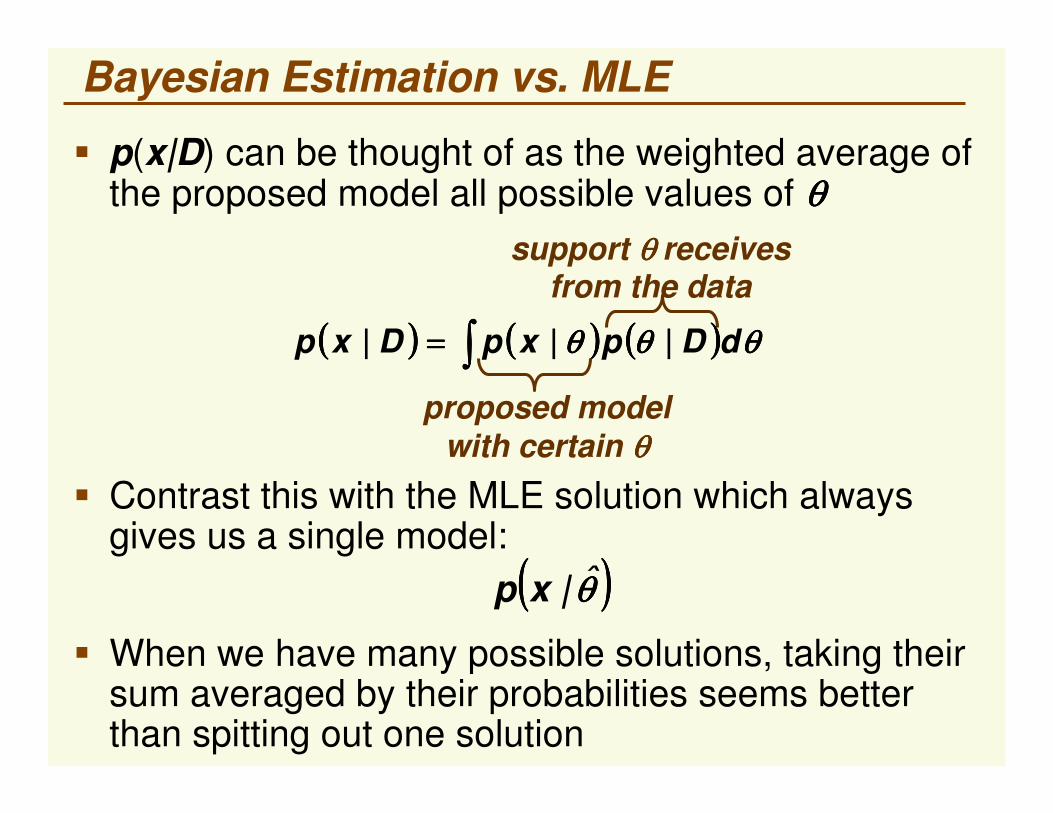
(((( )))) (((( )))) (((( ))))����==== θθθθθθθθθθθθ dDpxpDxp |||
� p(x|D) can be thought of as the weighted average of the proposed model all possible values of θθθθ
proposed model with certain θθθθ
support θ θ θ θ receives from the data
� Contrast this with the MLE solution which always gives us a single model:
(((( ))))θθθθ̂|xp
� When we have many possible solutions, taking their sum averaged by their probabilities seems better than spitting out one solution
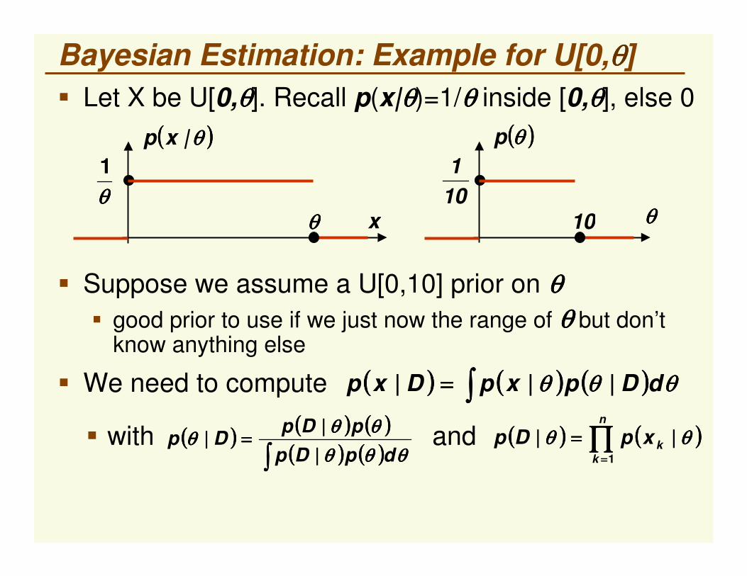
Bayesian Estimation: Example for U[0,θθθθ]� Let X be U[0,θθθθ]. Recall p(x|θθθθ)=1/θθθθ inside [0,θθθθ], else 0
(((( )))) (((( )))) (((( ))))����==== θθθθθθθθθθθθ dDpxpDxp |||
(((( )))) (((( )))) (((( ))))(((( )))) (((( ))))����
====θθθθθθθθθθθθ
θθθθθθθθθθθθdpDp
pDpDp
||
| (((( )))) (((( ))))∏∏∏∏====
====n
kkxpDp
1
|| θθθθθθθθ
� We need to compute
� with and
� Suppose we assume a U[0,10] prior on θθθθ� good prior to use if we just now the range of θθθθ but don’t
know anything else
θθθθθθθθ1
x 10101
θθθθ
(((( ))))θθθθp(((( ))))θθθθ|xp

Bayesian Estimation: Example for U[0,θθθθ](((( )))) (((( )))) (((( ))))����==== θθθθθθθθθθθθ dDpxpDxp |||
(((( )))) (((( )))) (((( ))))(((( )))) (((( ))))����
====θθθθθθθθθθθθ
θθθθθθθθθθθθdp|Dp
p|DpD|p (((( )))) (((( ))))∏∏∏∏
========
n
kkxpDp
1
|| θθθθθθθθ
� We need to compute
� using and
� When computing MLE of θθθθ, we had
(((( ))))��������
������������ ≥≥≥≥====
otherwise
xxforDp nn
0
},...,max{1
| 1θθθθθθθθθθθθ
� Thus
(((( ))))��������
������������ ≤≤≤≤≤≤≤≤====
otherwise0
10}x,...,xmax{for1
cD|p n1n θθθθθθθθθθθθ
� where c is the normalizing constant, i.e.
{{{{ }}}}����
==== 10
x...,xmaxn
n,1
d1
c
θθθθθθθθ
(((( ))))θθθθp
10101
θθθθ231 xxx
(((( ))))θθθθ|Dp

Bayesian Estimation: Example for U[0,θθθθ](((( )))) (((( )))) (((( ))))����==== θθθθθθθθθθθθ dDpxpDxp |||� We need to compute
(((( ))))��������
������������ ≤≤≤≤≤≤≤≤====
otherwise0
10}x,...,xmax{for1
cD|p n1n θθθθθθθθθθθθ
10 θθθθ231 xxx
(((( ))))D|p θθθθ
� We have 2 cases:1. case x < max{x1, x2,…, xn }
2. case x > max{x1, x2,…, xn }
(((( )))) ααααθθθθθθθθ
======== ���� ++++
10
}x,...xmax{ 1nn1
d1
cD|xp
θθθθ1
x
(((( ))))θθθθ|xp
θθθθ
(((( )))) nn10xn
10
x 1n 10nc
nxc
nc
d1
cD|xp −−−−====−−−−
======== ���� ++++ θθθθθθθθ
θθθθ
constant independent of x

Bayesian Estimation: Example for U[0,θθθθ]
(((( ))))D|xpBayes
231 xxx
x
� Note that even after x >max {x1, x2,…, xn }, Bayes density is not zero, which makes sense
10
αααα
(((( ))))θθθθ̂|xpML
� curious fact: Bayes density is not uniform, i.e. does not have the functional form that we have assumed!

ML vs. Bayesian Estimation with Broad Prior� Suppose p(θθθθ) is flat and broad (close to uniform prior)
� But by definition, peak of p(D|θθθθ) is the ML estimate θθθθ̂
� p(θθθθ|D) tends to sharpen if there is a lot of data
� Thus p(D|θθθθ) p(θθθθ|D)/p(θθθθ) will have the same sharp peak as p(θθθθ|D)
∝∝∝∝
(((( )))) (((( )))) (((( )))) (((( )))) (((( )))) (((( ))))θθθθθθθθθθθθθθθθθθθθθθθθθθθθ ˆ|xpdD|pˆ|xpdD|p|xpD|xp �������� ====≈≈≈≈====� The integral is dominated by the peak:
� Thus as n goes to infinity, Bayesian estimate will approach the density corresponding to the MLE!
(((( ))))θθθθ|Dp
(((( ))))D|p θθθθ
θθθθ̂
(((( ))))θθθθp
θθθθ θθθθ̂ θθθθ
(((( ))))θθθθ|xp
(((( ))))D|p θθθθ
(((( ))))θθθθ̂|xp
(((( ))))D|p θθθθ
θθθθ̂

ML vs. Bayesian Estimation: General Prior
� Maximum Likelihood Estimation� Easy to compute, use differential calculus� Easy to interpret (returns one model)� p(x|θθθθ) has the assumed parametric form
� Bayesian Estimation� Hard compute, need multidimensional integration� Hard to interpret, returns weighted average of
models� p(x|D) does not necessarily have the assumed
parametric form� Can give better results since use more
information about the problem (prior information)
^