1

Lecture 5:

BLUP (Best Linear Unbiased

Predictors) of genetic values

Bruce Walsh lecture notes

Tucson Winter Institute

9 - 11 Jan 2013

2

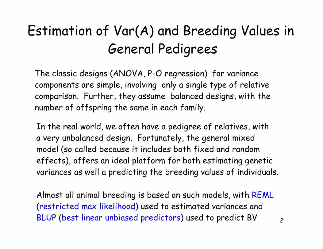
Estimation of Var(A) and Breeding Values in

General Pedigrees

The classic designs (ANOVA, P-O regression) for variance

components are simple, involving only a single type of relative

comparison. Further, they assume balanced designs, with the

number of offspring the same in each family.

In the real world, we often have a pedigree of relatives, with

a very unbalanced design. Fortunately, the general mixed

model (so called because it includes both fixed and random

effects), offers an ideal platform for both estimating genetic

variances as well a predicting the breeding values of individuals.

Almost all animal breeding is based on such models, with REML

(restricted max likelihood) used to estimated variances and

BLUP (best linear unbiased predictors) used to predict BV

3

BLUP in plant breeding• BLUP has migrated from animal breeding

into plant breeding.

• Advantages:– Handles unbalanced designs

– Uses information for all relatives measured toimprove estimates

• BLUP can be used to estimate a variety ofgenetic values– GCA, SCA, line values (i.e., genotypic values of

pure lines)

– One can also use BLUP machinery to estimateenvironmental effects

4

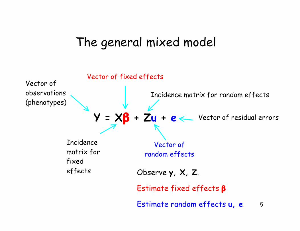
Y = X! + Zu + e

The general mixed model

Vector of

observations

(phenotypes)

Vector of fixed effects (to be estimated),

e.g., year, location and treatment effects

Vector of

random effects,

such as individual

genetic values

(to be estimated)

Vector of residual errors

(random effects)

Incidence

matrix for

fixed

effects

Incidence matrix for random effects

5

Y = X! + Zu + e

The general mixed model

Vector of

observations

(phenotypes)

Vector of

random effects

Incidence

matrix for

fixed

effects

Vector of fixed effects

Incidence matrix for random effects

Vector of residual errors

Observe y, X, Z.

Estimate fixed effects !

Estimate random effects u, e

6

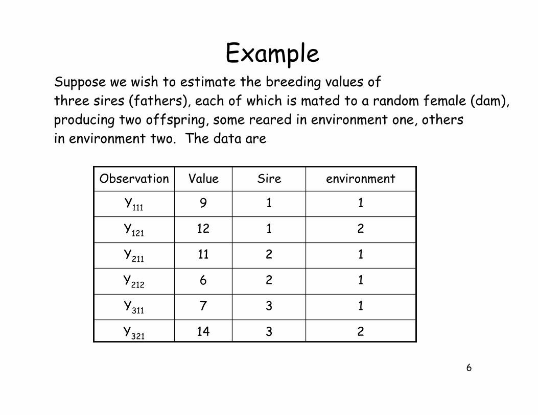
ExampleSuppose we wish to estimate the breeding values of

three sires (fathers), each of which is mated to a random female (dam),

producing two offspring, some reared in environment one, others

in environment two. The data are

2314Y321

137Y311

126Y212

1211Y211

2112Y121

119Y111

environmentSireValueObservation

7

y =

!

"""""#

y1,1,1

y1,2,1

y2,1,1

y2,1,2

y3,1,1

y3,2,1

$

%%%%%&=

!

"""""#

912116714

$

%%%%%&

X =

!

"""""#

1 00 11 01 01 00 1

$

%%%%%&, Z =

!

"""""#

1 0 01 0 00 1 00 1 00 0 10 0 1

$

%%%%%&, ! =

'!1

!2

(, u =

!

#u1

u2

u3

$

&

Here the basic model is

Yijk = !j + ui + eijk

Effect of environment jBreeding value of sire i

The mixed model vectors and

matrices become

8

Means: E(u) = E(e) = 0, E(y) = X!

Let R be the covariance matrix for the

residuals. We typically assume R = "2e*I

Let G be the covariance matrix for the

breeding values (the vector u)

The covariance matrix for y becomes

V = ZGZT + R

Means & Variances for y = X! + Zu + e

Variances:

9

)u = GZT V!1*y!X)!

+ -

)! = XT V!1X!1

XT V!1y

( )

Estimating fixed Effects & Predicting

Random Effects

For a mixed model, we observe y, X, and Z

!, u, R, and G are generally unknown

Two complementary estimation issues

(i) Estimation of ! and u

Estimation of fixed effects

Prediction of random effects

BLUE = Best Linear Unbiased Estimator

BLUP = Best Linear Unbiased Predictor

Recall V = ZGZT + R

10

Let’s return to our example

Assume residuals uncorrelated & homoscedastic,

R = "2e*I. Hence, need "2

e to solve BLUE/BLUP equations.

Suppose "2e = 6, giving R = 6* I

Now consider G, the covariance matrix for u (the vector

of the three sire breeding values). Assume the sires

are unrelated, so G is diagonal with element "2G = sire

variance, where "2G = "2

A /4.

Suppose "2A = 8, giving G G = 8/4*I

11

V =84

!

"""""#

1 0 01 0 00 1 00 1 00 0 10 0 1

$

%%%%%&

!

#1 0 00 1 00 0 1

$

&

!

#1 1 0 0 0 00 0 1 1 0 00 0 0 0 1 1

$

&+6

!

"""""#

1 0 0 0 0 00 1 0 0 0 00 0 1 0 0 00 0 0 1 0 00 0 0 0 1 00 0 0 0 0 1

$

%%%%%&

=

!

"""""#

8 2 0 0 0 02 8 0 0 0 00 0 8 2 0 00 0 2 8 0 00 0 0 0 8 20 0 0 0 2 8

$

%%%%%&giving V!1 =

130

·

!

"""""#

4 !1 0 0 0 0!1 4 0 0 0 0

0 0 4 !1 0 00 0 !1 4 0 00 0 0 0 4 !10 0 0 0 !1 4

$

%%%%%&-

-

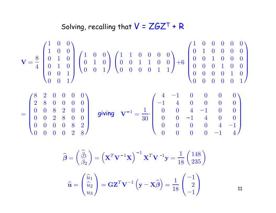
Solving, recalling that V = ZGZT + R

)! =' )!1

)!2

(=

*XTV!1X

+!1XTV 1y =

118

'148235

(

)u =

!

#)u1

)u2

u3

$

& = GZTV!1*y!X)!

+=

118

!

#!1

2!1

$

&

- - -

12

BLUP estimates of line valuesBernardo example (11.3.1): yield in four (related) inbred lines of

Barley raised over two sets of environments

Model

Environment type

(fixed)

Line value

(random)

)

13

bi = µ + ti

Line values

Relationship values (from pedigree

data on how lines are related)

Observations differ in their residual

error due to sample size differences

14

!

#XTR!1X XTR!1Z

ZTR!1X ZTR!1Z + G!1

$

&

!

#)!

)u

$

& =

!

#XTR!1y

ZTR!1y

$

&

Henderson’s Mixed Model Equations

)! = XT V!1X!1

XT V!1y

( )

)u = GZT V!1*y!X)!

+

If X is n x p and Z is n x q

Inversion of an n x n matrix

p x p p x q

q x q

The whole matrix is (p+q) x (p+q)

y = X! + Zu + e, u ~ (0,G), e ~ (0, R), cov(u,e) = 0,

V = ZGZT + R

q x pq

Easier to numerically work

with than BLUP/BLUE

equations

15

16

Let’s redo our example on slide 6

using Henderson’s Equation

XTR!1X =16

'4 00 2

(, XTR!1Z =

*ZTR!1X

+T=

16

'1 2 11 0 1

(

G!1+ZTR!1Z =56

!

#1 0 00 1 00 0 1

$

& , XTR!1y =16

'3326

(, ZTR!1y =

16

!

#211721

$

&

!

"""#

4 0 1 2 10 2 1 0 11 1 5 0 02 0 0 5 01 1 0 0 5

$

%%%&

!

""""#

)!1)!2

)u1

)u2

)u3

$

%%%%&=

!

"""#

3326211721

$

%%%&

Taking the inverse gives

!

""""#

)!1)!2

)u1

)u2

)u3

$

%%%%&=

118

!

"""#

148235!1

2!1

$

%%%&

As found above

17

The Animal Model, yi = µ + ai + ei

!

#

$

&

!

#

$

X =""

11...1

%% , ! = µ, u =""

a1

a2...

ak

%%& G = "2A A,

Here, the individual is the unit of analysis, with

yi the phenotypic value of the individual and ai its BV

Where the additive genetic relationship matrix A is given by

Aij = 2#ij, ,namely twice the coefficient of coancestry

Assume R = "2e*I, so that R-1 = 1/("2

e)*I.

Likewise, G = "2A*A, so that G-1 = 1/("2

A)*A-1.

The “animal” model estimates the breeding value for each

individual, even for a plant or tree! Same approach also

works to estimate line (genotypic) values for inbreds.

18

!

#XTX XTZ

ZTX ZTZ + #A!1

$

&

!

#)!

)u

$

& =

!

#XTy

ZTy

$

&

!

#n 1T

1 I + #A!1

$

&

!

#)µ

)u

$

& =

!

#

,nyi

y

$

&

Henderson’s mixed model equations

This reduces to

here $ = "2e / "2

A = (1-h2)/h2

Returning to the animal model

19

Example

1 2 3

4 5

Suppose our pedigree is

A =

!

"""#

1 0 0 1/2 00 1 0 1/2 1/20 0 1 0 1/2

1/2 1/2 0 1 1/40 1/2 1/2 1/4 1

$

%%%&

I + #A!1 =

!

"""#

5/2 1/2 0 !1 01/2 3 1/2 !1 !1

0 1/2 5/2 0 !1!1 !1 0 3 0

0 !1 !1 0 3

$

%%%&

Suppose $ =1 (corresponds to h2 = 0.5). In this case,

20

!

"""""#

5 1 1 1 1 11 5/2 1/2 0 !1 01 1/2 3 1/2 !1 !11 0 1/2 5/2 0 11 1 !1 0 3 01 0 !1 !1 0 3

$

%%%%%&

!

"""""#

)µ)a1

)a2

)a3

)a4

)a5

$

%%%%%&=

!

"""""#

41791069

$

%%%%%&--

))µ =44053

" 8.302,

!

"""#

)a1

)a2

)a3

)a4

a5

$

%%%& =

!

"""#

!662/6894/53

610/689!732/689

381/689

$

%%%& "

!

"""#

!0.9610.0760.885!1.062

0.553

$

%%%&

Suppose the vector of

observations isy =

!

"""#

y1

y2

y3

y4

y5

$

%%%& =

!

"""#

791069

$

%%%&

Here n = 5, % y = 41, and Henderson’s equation becomes

Solving gives

21

More on the animal model• Under the animal model

– y = X! + Za + e

– a ~ (0,"A2A), e ~ (0, "e

2I)

– BLUP(a) = "A2AZTV-1(y- X!)

– Where V = ZGZT + R = "A2ZAZT + "e

2I

• Consider the simplest case of a single observationon one individual, where the only fixed effect isthe mean µ, which is assumed known

– Here Z = A = I = (1),

– V = "A2 + "e

2

– "A2 AZTV-1 = "A

2 /("A2 + "e

2) = h2

– BLUP(a) = h2(y-µ)

22

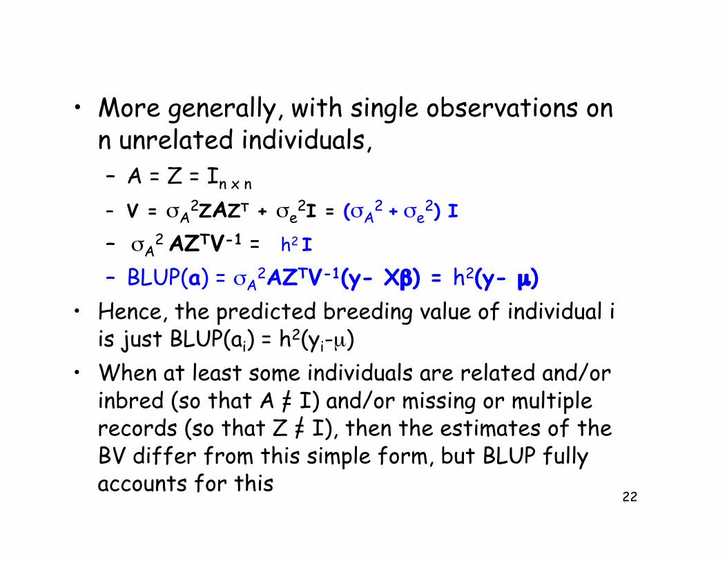
• More generally, with single observations onn unrelated individuals,– A = Z = In x n

– V = "A2ZAZT + "e

2I = ("A2 + "e

2) I

– "A2 AZTV-1 = h2 I

– BLUP(a) = "A2AZTV-1(y- X!) = h2(y- µ)

• Hence, the predicted breeding value of individual iis just BLUP(ai) = h2(yi-µ)

• When at least some individuals are related and/orinbred (so that A = I) and/or missing or multiplerecords (so that Z = I), then the estimates of theBV differ from this simple form, but BLUP fullyaccounts for this

23

BLUP is a shrinkage estimator

• For a single observation on one individual,BLUP(a) = h2(y-µ)– The difference between the observed value (y)

and the mean (µ) is shrunk by the factor h2 ---shrinks the estimate back towards the mean(zero in the case of BVs)

• More generally, BLUP(a) = GZTV-1(y- X!)

– First adjusts observations (y) for fixed effects(X!) and then regresses this difference backtowards zero (the mean BV), as Cov*Var-1 is ageneralized regression coefficient

24

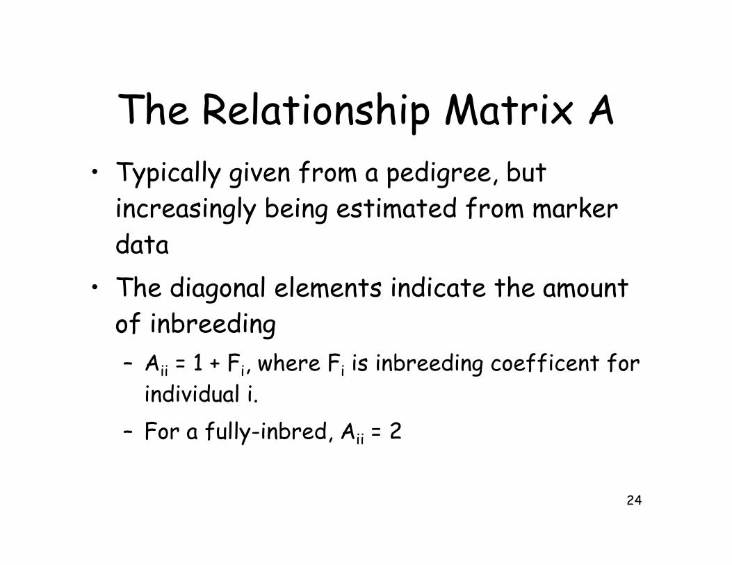
The Relationship Matrix A

• Typically given from a pedigree, but

increasingly being estimated from marker

data

• The diagonal elements indicate the amount

of inbreeding

– Aii = 1 + Fi, where Fi is inbreeding coefficent for

individual i.

– For a fully-inbred, Aii = 2

25

Marker-based relationship matrices• There are two reasons for using a marker-

estimated relationship matrix– Pedigree either unknown or poorly known

– With very dense markers, provides a better estimatethan a known pedigree. Why?

• Consider two (non-inbred) full-sibs. The expectationunder a pedigree is that they share exactly half theirgenes.

• However, there is a sampling variance about thisexpected value, so that some pair of sibs may sharemore than 50%, while another may share less. Usingmarkers to detect such pairs improves the estimatedvalues

• This is called G-BLUP (in animal breeding) and is aform of genomic selection

26

Marker-based relationship matrix

Simplest case is to consider a very large number (L) of SNPs, and

treat alike in state as IBD, and then compute the probability

fxy that x and y share a randomly-drawn allele for each SNP marker.

Twice the average over all markers is the entry for x and y in the

relationship matrix (as Axy = 2fxy)

10.5011

0.50.50.501

00.5100

110100

SNP genotype for x

SN

P ge

noty

pe f

or y

Values for fxy given the SNP genotypes

27

Estimation of R and G

A second estimation issue concerns the covariance

matrix for residuals R and for breeding values G

As we have seen, both matrices have the form

"2*B, where the variance "2 is unknown, but

B is known

For example, for residuals, R = "2e*I

For breeding values, G = "2A*A, where A is given

from the pedigree

28

REML Variance Component Estimation

REML = Restricted Maximum Likelihood.

REML maximizes that portion of the likelihood that

does not depend on fixed effects

Standard ML variance estimation assumes fixed

factors are known without error. Results in downward

bias in variance estimates

Basic idea: Use a transformation to remove fixed

effect, then perform ML on this transformed vector

29

Simple variance estimate under ML vs. REML

ML =1n

n-

i+1

(x! x)2, REML =1

n! 1

n-

i+1

(x! x)2

REML adjusts for the

estimated fixed

effect,

in this case, the mean

With balanced design, ANOVA variance estimates are

equivalent to REML variance estimates

30

Multiple random effects

y = X! + Za + Wu + e

! is a q x 1 vector of fixed effects

a is a p x 1 vector of random effects

u is a m x 1 vector of random effects

X is n x q, Z is n x p, W is n x m

y is a n x 1 vector of observations

y, X, Z, W observed. !, a, u, e to be estimated

31

Covariance structure

Defining the covariance structure key in any mixed-model

y = X! + Za + Wu + e

These covariances matrices are still not sufficient, as we

have yet to give describe the relationship between e, a,

and u. If they are independent:

Suppose e ~ (0,"e2 I), u ~ (0,"u

2 I), a ~ (0,"A2 A),

as with breeding values

32

y = X! + Za + Wu + e

Note that if we ignored the second vector u of random

effects, and assumed y = X! + Za + e*, then e* =

Wu + e, with Var(e*) = "e2 I + "u

2 WWT

Consequence of ignoring random effects is that these

are incorporated into the residuals, potentially

compromising its covariance structure

Covariance matrix for the vector of observations y

33

Mixed-model Equations

34

The repeatability model

• Often, multiple measurements (aka “records”) are collected onthe same individual

• Such a record for individual k has three components

– Breeding value ak

– Common (permanent) environmental value pk

– Residual value for ith observation eki

• Resulting observation is thus

– zki = µ + ak + pk +eki

• The repeatability of a trait is r = ("A2+"p

2)/"z2

• Resulting variance of the residuals is "e2 = (1-r) "z

2

35

Resulting mixed model

y = X! + Za + Zp + e

In class question: Why can we obtain separate estimates

of a and p?

Notice that we could also write this model as

y = X! + Z(a + p) + e = y = X! + Zv + e, v = a+p

36

37

The incident matrix ZSuppose we have a total of 7 observations/records, with

3 measures from individual 1, 2 from individual 2, and

2 from individual 3. Then:

Why? Matrix multiplication. Consider y21.

y21 = µ + A2 + p2 + e21

38

Consequences of ignoring p• Suppose we ignored the permanent environment effects and

assumed the model y = X! + Za + e*

– Then e* = Zp + e,

– Var(e*) = "e2 I + "p

2 ZZT

• Assuming that Var(e*) = "e2 I gives an incorrect model

• We could either– use y = X! + Za + e* with the correct error structure

(covariance) for e* = "e2 I + "p

2 ZZT

– Or use y = X! + Za +Zp + e, where e = "e2 I

39

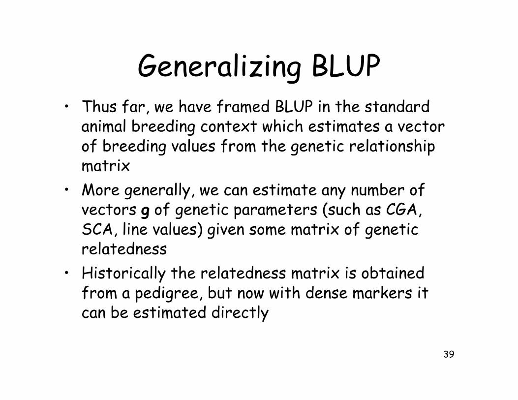
Generalizing BLUP• Thus far, we have framed BLUP in the standard

animal breeding context which estimates a vectorof breeding values from the genetic relationshipmatrix

• More generally, we can estimate any number ofvectors g of genetic parameters (such as CGA,SCA, line values) given some matrix of geneticrelatedness

• Historically the relatedness matrix is obtainedfrom a pedigree, but now with dense markers itcan be estimated directly

40

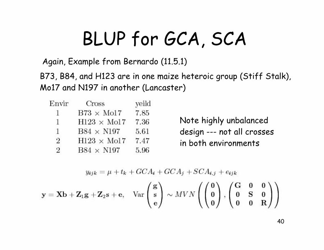
BLUP for GCA, SCAAgain, Example from Bernardo (11.5.1)

B73, B84, and H123 are in one maize heteroic group (Stiff Stalk),

Mo17 and N197 in another (Lancaster)

Note highly unbalanced

design --- not all crosses

in both environments

41

Covariance matrix based on pedigree information (see Bernardo

for details)