Lecture 4

The L2 Normand

Simple Least Squares

SyllabusLecture 01 Describing Inverse ProblemsLecture 02 Probability and Measurement Error, Part 1Lecture 03 Probability and Measurement Error, Part 2 Lecture 04 The L2 Norm and Simple Least SquaresLecture 05 A Priori Information and Weighted Least SquaredLecture 06 Resolution and Generalized InversesLecture 07 Backus-Gilbert Inverse and the Trade Off of Resolution and VarianceLecture 08 The Principle of Maximum LikelihoodLecture 09 Inexact TheoriesLecture 10 Nonuniqueness and Localized AveragesLecture 11 Vector Spaces and Singular Value DecompositionLecture 12 Equality and Inequality ConstraintsLecture 13 L1 , L∞ Norm Problems and Linear ProgrammingLecture 14 Nonlinear Problems: Grid and Monte Carlo Searches Lecture 15 Nonlinear Problems: Newton’s Method Lecture 16 Nonlinear Problems: Simulated Annealing and Bootstrap Confidence Intervals Lecture 17 Factor AnalysisLecture 18 Varimax Factors, Empircal Orthogonal FunctionsLecture 19 Backus-Gilbert Theory for Continuous Problems; Radon’s ProblemLecture 20 Linear Operators and Their AdjointsLecture 21 Fréchet DerivativesLecture 22 Exemplary Inverse Problems, incl. Filter DesignLecture 23 Exemplary Inverse Problems, incl. Earthquake LocationLecture 24 Exemplary Inverse Problems, incl. Vibrational Problems

Purpose of the Lecture

Introduce the concept of prediction error and the norms that quantify it

Develop the Least Squares Solution

Develop the Minimum Length Solution

Determine the covariance of these solutions

Part 1

prediction error and norms

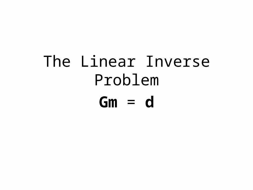
The Linear Inverse ProblemGm = d

The Linear Inverse ProblemGm = ddatamodel

parameters

data kernel

Gmest = dprean estimate of the model parameters can be

used to predict the data

but the prediction may not match the observed data

(e.g. due to observational error)dpre ≠ dobs

e = dobs -dprethis mismatch leads us to define the

prediction error

e = 0when the model parameters exactly predict the data

B)A)

0 5 100

5

10

15

z

d

0 5 100

5

10

15

z

d

zi

diobsdipre ei

example of prediction errorfor line fit to data

“norm”rule for quantifying the overall size

of the error vector elot’s of possible ways to do it

Ln family of norms

Ln family of norms

Euclidian length

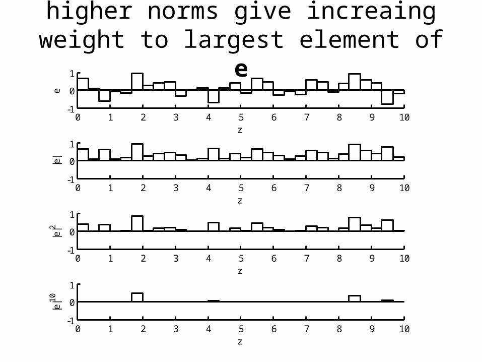
0 1 2 3 4 5 6 7 8 9 10-1

0

1

z

e

0 1 2 3 4 5 6 7 8 9 10-1

0

1

z

|e|

0 1 2 3 4 5 6 7 8 9 10-1

0

1

z

|e|2

0 1 2 3 4 5 6 7 8 9 10-1

0

1

z

|e|10

higher norms give increaing weight to largest element of e

limiting case

guiding principle for solving an inverse problem

find the mest

that minimizes E=||e||

withe = dobs –dpreand dpre = Gmest

but which norm to use?

it makes a difference!

0 2 4 6 8 100

5

10

15

z

d

outlier

L1L2

L∞

B)A)

0 5 100

0.1

0.2

0.3

0.4

0.5

d

p(d)

0 5 100

0.1

0.2

0.3

0.4

0.5

d

p(d)

Answer is related to the distribution of the error. Are outliers common or rare?

long tailsoutliers common

outliers unimportantuse low norm

gives low weight to outliers

short tailsoutliers uncommonoutliers important

use high normgives high weight to outliers

as we will show later in the class …

use L2 norm when data has

Gaussian-distributed error

Part 2

Least Squares Solution to Gm=d

L2 norm of error is its Euclidian length

so E is the square of the Euclidean lengthmimimize E

Principle of Least Squares

= eTe

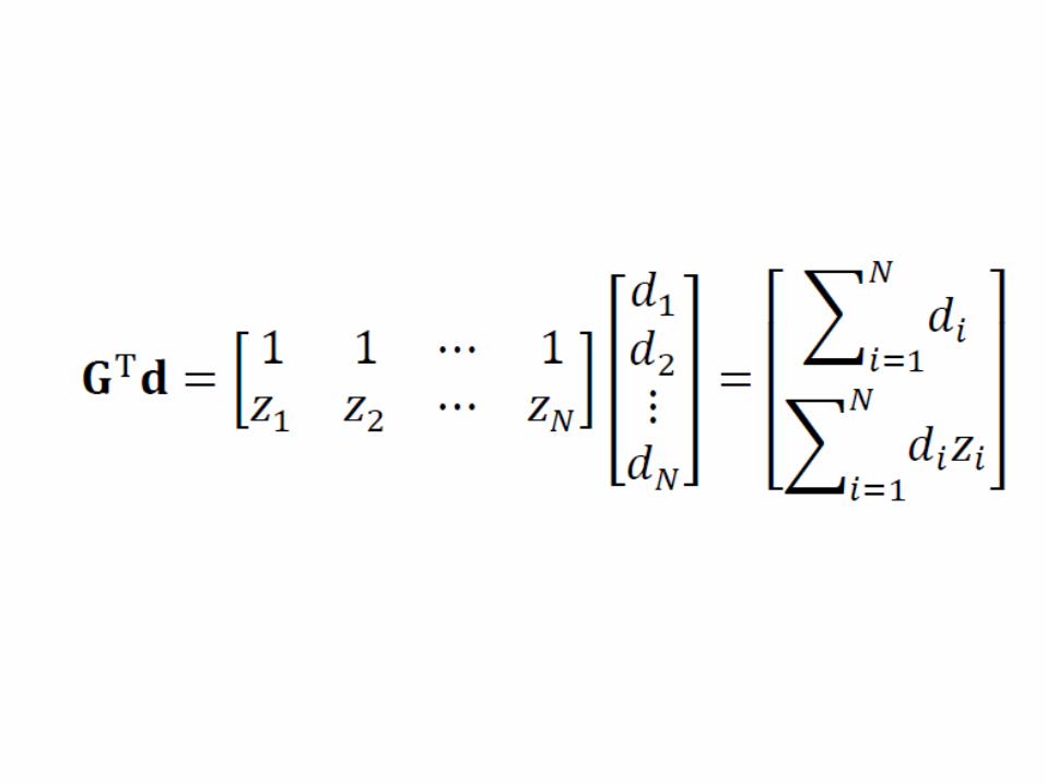
Least Squares Solution to Gm=d

minimize E with respect to mq∂E/∂mq = 0

so, multiply out

first term

first term

∂mj /∂mq = δjq since mj and mq are independent variables

ai = Σj δij bj = bi

Kronecker delta(elements of identity matrix) [I]ij = δij

a = Ib = bai = Σj δij bj = bi

i

second term

third term

putting it all together

or

presuming [GTG] has an inverse

Least Square Solution

presuming [GTG] has an inverse

Least Square Solution

memorize

examplestraight line problem

Gm = d

in practice,no need to multiply matrices

analytically

just use MatLab

mest = (G’*G)\(G’*d);

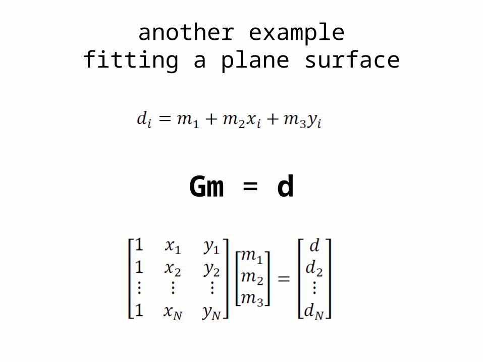
another examplefitting a plane surface

Gm = d

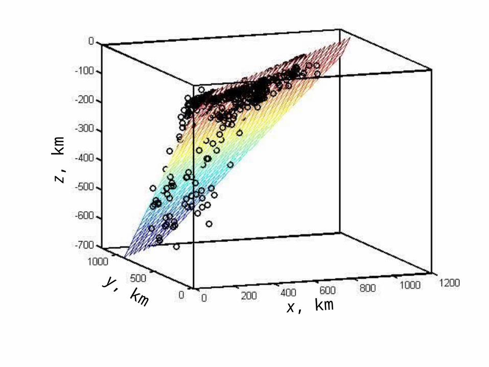
x, km

y, km

z, km

Part 3

Minimum Length Solution

but Least Squares will fail

when [GTG] has no inverse

zd

?

?

?

examplefitting line to a single point

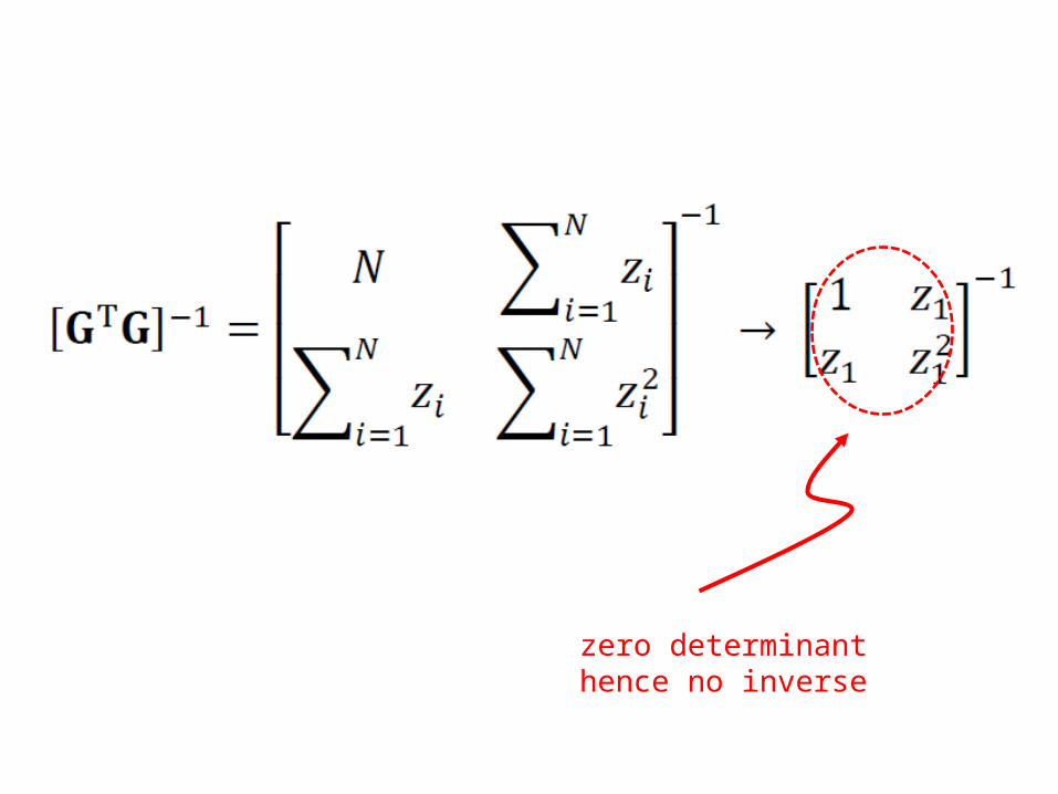
zero determinanthence no inverse

Least Squares will fail

when more than one solution minimizes the error

the inverse problem is “underdetermined”

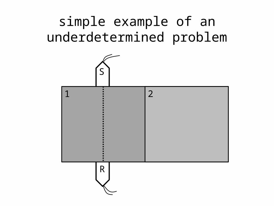
R

S

21

simple example of an underdetermined problem

What to do?

use another guiding principle

“a priori” information about the solution

in the casechoose a solution that is small

minimize ||m||2

simplest case“purely underdetermined”

more than one solution has zero error

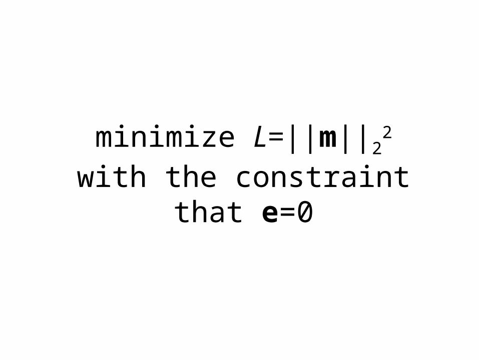
minimize L=||m||22with the constraint that e=0

Method of Lagrange Multipliersminimize L with constraintsC1=0, C2=0, …

equivalent to

minimize Φ=L+λ1C1+λ2C2+…with no constraints λs called “Lagrange Multipliers”

e(x,y)=0

x

y

L (x,y)(x0,y0)

2m=GT λ and Gm=d G½ GT λ =d

λ = 2[GGT ]-1d m=GT [GGT ]-1d

presuming [GGT] has an inverse

Minimum Length Solution

mest=GT [GGT ]-1d

presuming [GGT] has an inverse

Minimum Length Solution

mest=GT [GGT ]-1dmemorize

Part 4

Covariance

Least Squares Solutionmest= [GTG ]-1GTdMinimum Length Solutionmest=GT [GGT ]-1dboth have the linear formm=Md

but ifm=Mdthen[cov m] = M [cov d] MT

when data are uncorrelated with uniform variance σd2

[cov d]=σd2I

so

Least Squares Solution[cov m] = [GTG ]-1GTσd2 G[GTG ]-1[cov m] = σd

2 [GTG ]-1

Minimum Length Solution[cov m] = GT [GGT ]-1 σd2 [GGT ]-1G[cov m] = σd

2 GT [GGT ]-2G

Least Squares Solution[cov m] = [GTG ]-1GTσd2 G[GTG ]-1[cov m] = σd

2 [GTG ]-1

Minimum Length Solution[cov m] = GT [GGT ]-1 σd2 [GGT ]-1G[cov m] = σd

2 GT [GGT ]-2G memorize

where to obtain the value of σd2 a priori value – based on knowledge of accuracy

of measurement technique

my ruler has 1 mm divisions, so σd≈ mm½

a posteriori value – based on prediction error

variance critically dependent on experiment design (structure of G)

1 12 123

1234

1 12 23 34… …

which is the better way to weigh a set of boxes ?

0 10 20 30 40 50 60 70 80 90 100

-2

0

2m

z

0 10 20 30 40 50 60 70 80 90 1000

0.5

1

sm

z

A)

B)

miest

σmi

i

i

0 1 2 3 4

0

1

2

3

4

500

1000

1500

2000

0 1 2 3 4

0

1

2

3

4

500

1000

1500

2000

2500

3000

-5 0 5-10

-5

0

5

10

-5 0 5-10

-5

0

5

10

-5 0 5-10

-5

0

5

10

-5 0 5-10

-5

0

5

10

z

m1

m20 40

4m1

0

4

m20 4E Ezd d

A) B)

C) D)

Relationship between[cov m] and Error Surface

Taylor Series expansion of the error about its minimum

Taylor Series expansion of the error about its minimum

curvature matrixwith elements∂2E/ ∂mi∂mj

for a linear problemcurvature is related to GTGE = (Gm-d)T(Gm-d) =

mT[GTG]m-dTGm-mTGTd+dTdso

∂2E/ ∂mi∂mj = [GTG] ij

and since

[cov m] = σd2 [GTG]-1we have

the sharper the minimumthe higher the curvature

the smaller the covariance