Lecture 4 - 1 ERS 482/682 (Fall 2002) Precipitation ERS 482/682 Small Watershed Hydrology.
45
ERS 482/682 (Fall 2002) Lecture 4 - 1 Precipitation ERS 482/682 Small Watershed Hydrology
-
date post
19-Dec-2015 -
Category
Documents
-
view
217 -
download
0
Transcript of Lecture 4 - 1 ERS 482/682 (Fall 2002) Precipitation ERS 482/682 Small Watershed Hydrology.
ERS 482/682 (Fall 2002) Lecture 4 - 1
Precipitation
ERS 482/682Small Watershed Hydrology
ERS 482/682 (Fall 2002) Lecture 4 - 2
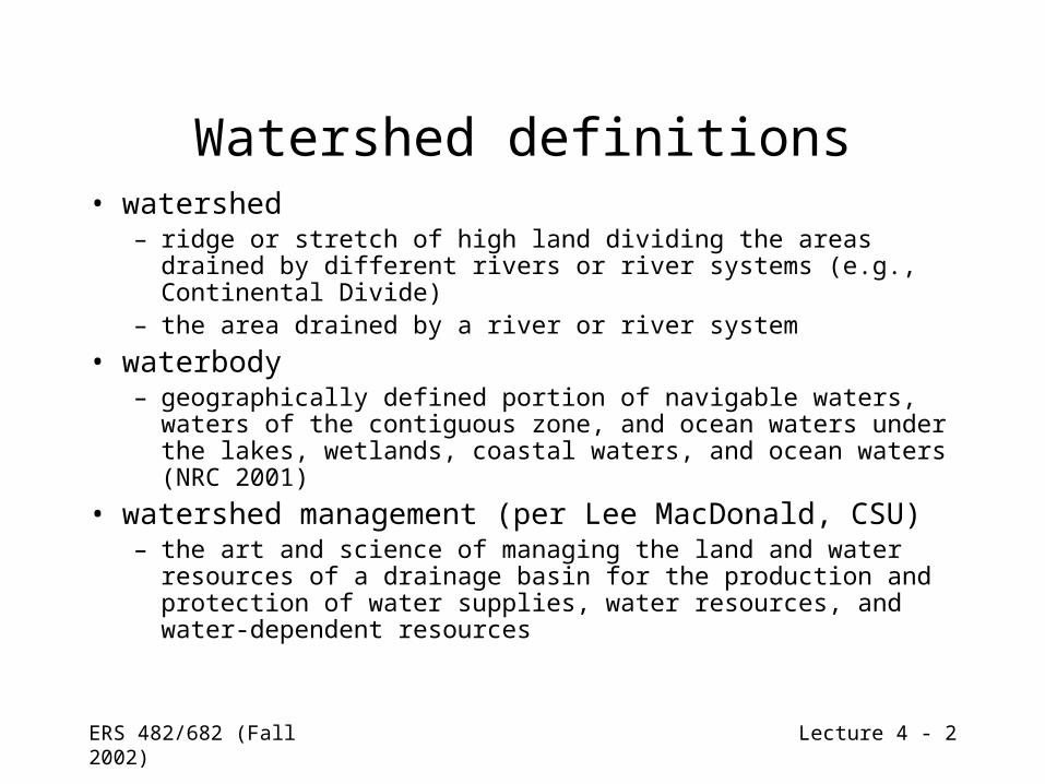
Watershed definitions• watershed
– ridge or stretch of high land dividing the areas drained by different rivers or river systems (e.g., Continental Divide)
– the area drained by a river or river system
• waterbody– geographically defined portion of navigable waters,
waters of the contiguous zone, and ocean waters under the lakes, wetlands, coastal waters, and ocean waters (NRC 2001)
• watershed management (per Lee MacDonald, CSU)– the art and science of managing the land and water
resources of a drainage basin for the production and protection of water supplies, water resources, and water-dependent resources
ERS 482/682 (Fall 2002) Lecture 4 - 3
Precipitation
• Water that falls to the earth (and reaches it)– Rain– Snow– Ice pellets (sleet)– Hail– Drizzle
ERS 482/682 (Fall 2002) Lecture 4 - 4
Process of precipitation
• Global circulation• Formation of precipitation
– uplift– temperature
ERS 482/682 (Fall 2002) Lecture 4 - 5
Global circulation
• Distribution of solar radiation intensity
Figure 3-4: Dingman (2002)
ERS 482/682 (Fall 2002) Lecture 4 - 6
Global circulation
• Earth’s rotation
Figure 4.1: Manning (1987)

ERS 482/682 (Fall 2002) Lecture 4 - 7
Formation of precipitation
• Water vapor importation• Cooling of air to
dewpoint temperature• Condensation• Growth of droplets or
crystals
See Appendix D for more detail
ERS 482/682 (Fall 2002) Lecture 4 - 8
Air cooling
• Cyclonic uplift
Figures 4.2 and 4.3: Manning (1987)
ERS 482/682 (Fall 2002) Lecture 4 - 9
Air cooling
• Thunderstorm uplift
Figure 4.4: Manning (1987) Figure 4-7: Dingman (2002)
ERS 482/682 (Fall 2002) Lecture 4 - 10
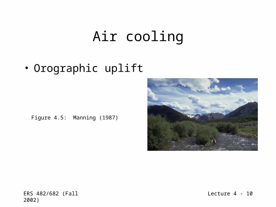
Air cooling
• Orographic uplift
Figure 4.5: Manning (1987)
ERS 482/682 (Fall 2002) Lecture 4 - 11
Condensation
Figure 2.1: Hornberger et al. (1998)
ERS 482/682 (Fall 2002) Lecture 4 - 12
CondensationAssumption:Pressure isconstant
Figure 2.1: Hornberger et al. (1998)
ERS 482/682 (Fall 2002) Lecture 4 - 13
Formation of droplets
Figure D-7: Dingman (2002)
Condensation requires condensation nuclei
ERS 482/682 (Fall 2002) Lecture 4 - 14
Measuring precipitation
• Units– Depth (L)– Intensity (L T-1)
Figure 2-2; Dunneand Leopold
(1978)
ERS 482/682 (Fall 2002) Lecture 4 - 15
Precipitation characteristics
• Typical precipitation intensities <1”/hr• General rule: longer storm duration
lower average intensity
ERS 482/682 (Fall 2002) Lecture 4 - 16
Figure 4-51 (a): Dingman (2002)
ERS 482/682 (Fall 2002) Lecture 4 - 17
Figure 4-51(c): Dingman (2002)

ERS 482/682 (Fall 2002) Lecture 4 - 18
Precipitation characteristics
• Typical precipitation intensities <1”/hr• General rule: longer storm duration
lower average intensity• Larger area lower average intensity
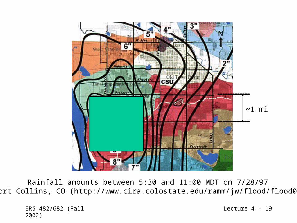
ERS 482/682 (Fall 2002) Lecture 4 - 19
Rainfall amounts between 5:30 and 11:00 MDT on 7/28/97for Fort Collins, CO (http://www.cira.colostate.edu/ramm/jw/flood/flood0.htm)
~1 mi
ERS 482/682 (Fall 2002) Lecture 4 - 20
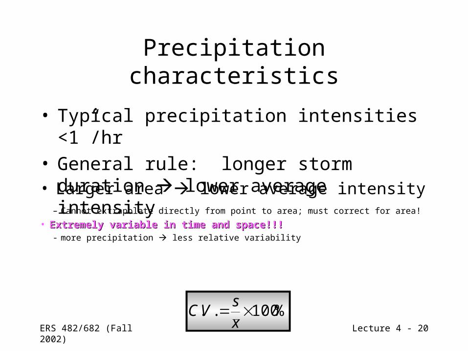
Precipitation characteristics
• Typical precipitation intensities <1”/hr• General rule: longer storm duration
lower average intensity• Larger area lower average intensity
– Cannot extrapolate directly from point to area; must correct for area!
• Extremely variable in time and space!!!Extremely variable in time and space!!!- more precipitation less relative variability
%100.. xs
VC
ERS 482/682 (Fall 2002) Lecture 4 - 21
Precipitation-gage networks
• World Meteorological Association recommendations: Table 4-6 (Dingman text)
• Need ~ 1 gage every km2 (250 acres) to get error under ~10%
ERS 482/682 (Fall 2002) Lecture 4 - 22
Figure 4-31Dingman text
ERS 482/682 (Fall 2002) Lecture 4 - 23
Precision
• Precision improves with:– Increasing density of gage network– Extending period of measurement– Increase in time and cost!
How close can we get to the true value?
ERS 482/682 (Fall 2002) Lecture 4 - 24
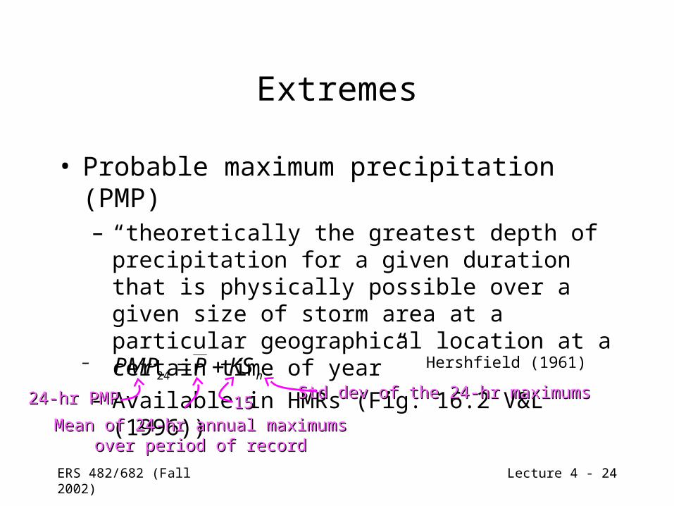
• Probable maximum precipitation (PMP)– “theoretically the greatest depth of
precipitation for a given duration that is physically possible over a given size of storm area at a particular geographical location at a certain time of year”
– Available in HMRs (Fig. 16.2 V&L (1996))
Extremes
– Hershfield (1961)nKSPPMP 24
24-hr PMP24-hr PMP
Mean of 24-hr annual maximumsMean of 24-hr annual maximumsover period of recordover period of record
1515 Std dev of the 24-hr maximumsStd dev of the 24-hr maximums
ERS 482/682 (Fall 2002) Lecture 4 - 25
Extremes
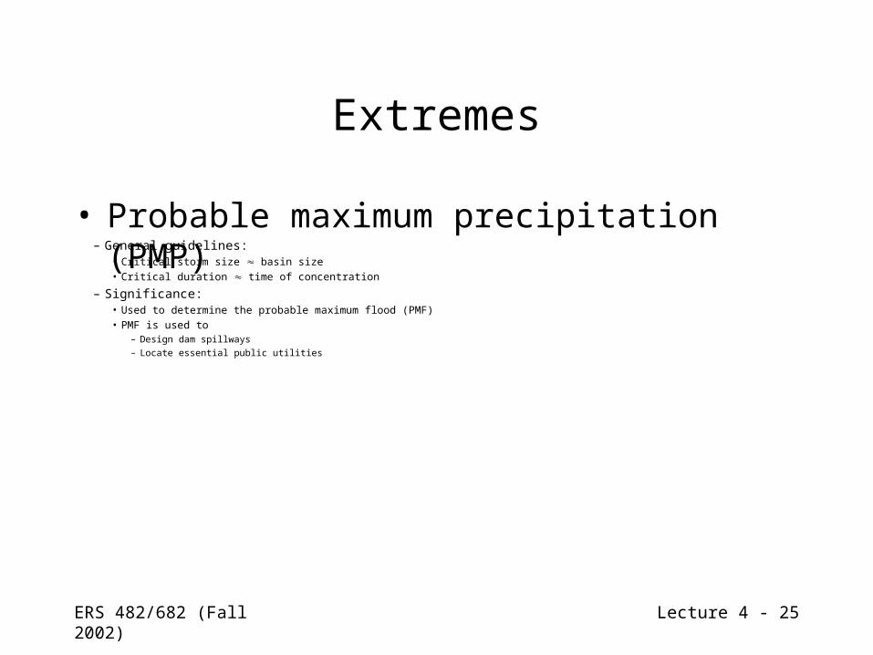
• Probable maximum precipitation (PMP)– General guidelines:
• Critical storm size basin size• Critical duration time of concentration
– Significance:• Used to determine the probable maximum flood (PMF)• PMF is used to
– Design dam spillways– Locate essential public utilities
ERS 482/682 (Fall 2002) Lecture 4 - 26
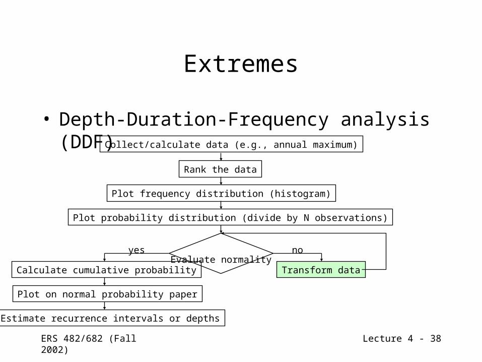
Extremes
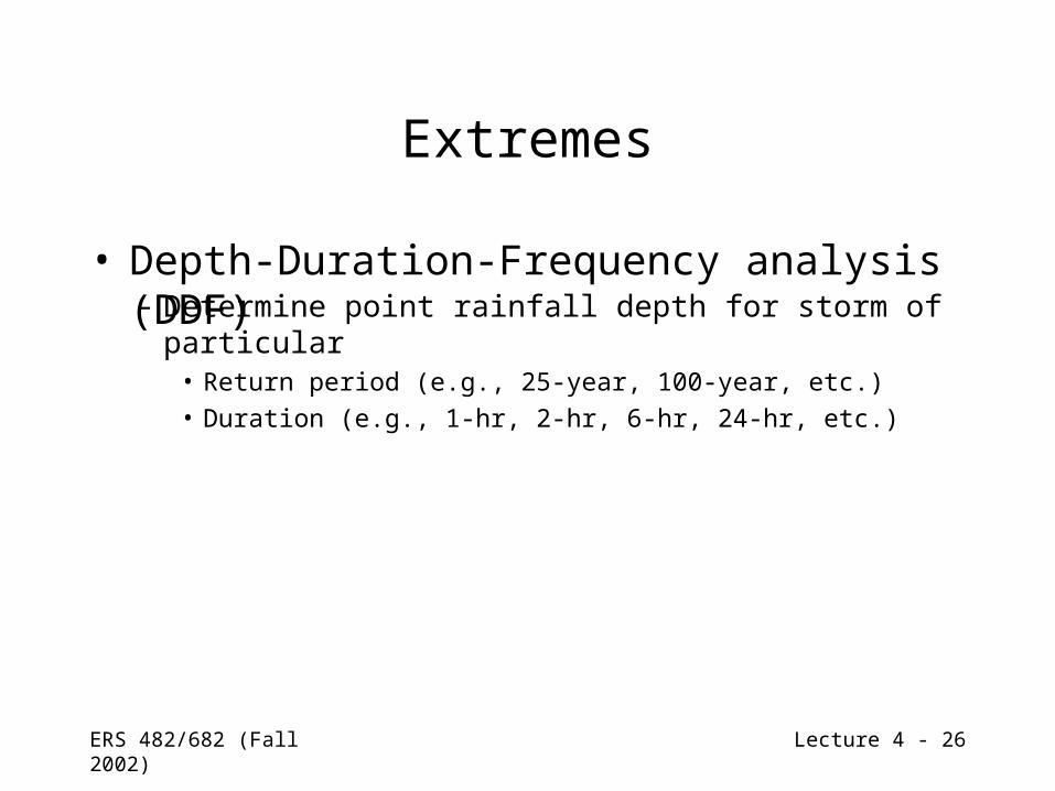
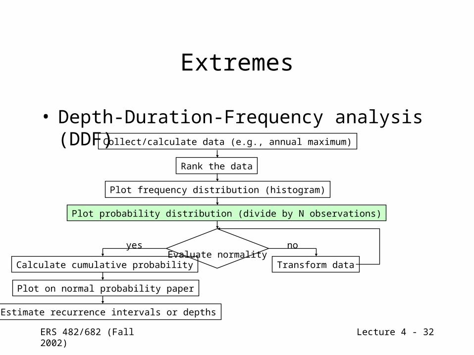
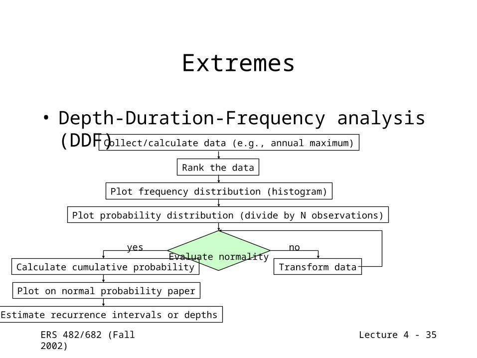
• Depth-Duration-Frequency analysis (DDF)– Determine point rainfall depth for storm of
particular• Return period (e.g., 25-year, 100-year, etc.)• Duration (e.g., 1-hr, 2-hr, 6-hr, 24-hr, etc.)
ERS 482/682 (Fall 2002) Lecture 4 - 27
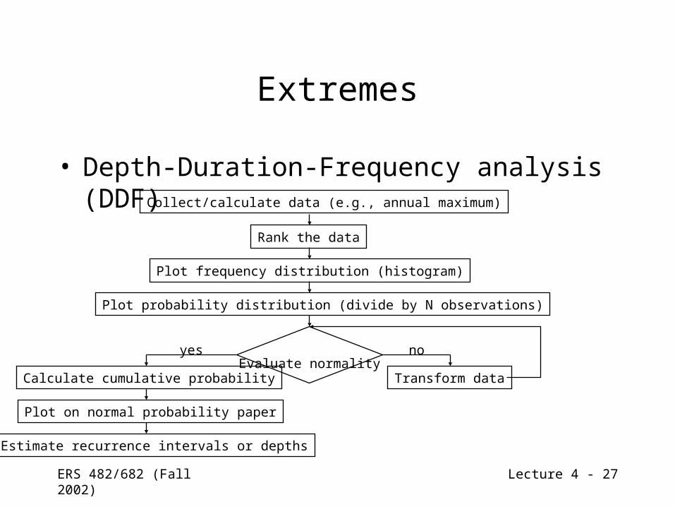
Extremes
• Depth-Duration-Frequency analysis (DDF) Collect/calculate data (e.g., annual maximum)
Rank the data
Plot frequency distribution (histogram)
Plot probability distribution (divide by N observations)
Evaluate normalityCalculate cumulative probability
Plot on normal probability paper
Estimate recurrence intervals or depths
Transform data
yes no
ERS 482/682 (Fall 2002) Lecture 4 - 28
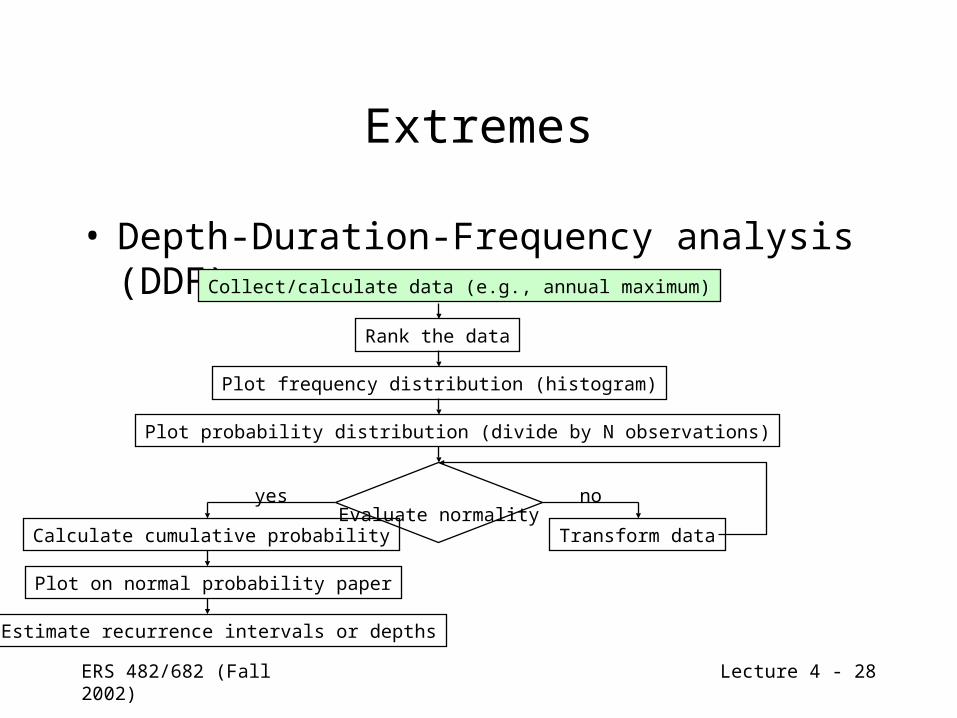
Extremes
• Depth-Duration-Frequency analysis (DDF) Collect/calculate data (e.g., annual maximum)
Rank the data
Plot frequency distribution (histogram)
Plot probability distribution (divide by N observations)
Evaluate normalityCalculate cumulative probability
Plot on normal probability paper
Estimate recurrence intervals or depths
Transform data
yes no

ERS 482/682 (Fall 2002) Lecture 4 - 29
Extremes
• Depth-Duration-Frequency analysis (DDF) Collect/calculate data (e.g., annual maximum)
Rank the data
Plot frequency distribution (histogram)
Plot probability distribution (divide by N observations)
Evaluate normalityCalculate cumulative probability
Plot on normal probability paper
Estimate recurrence intervals or depths
Transform data
yes no
ERS 482/682 (Fall 2002) Lecture 4 - 30
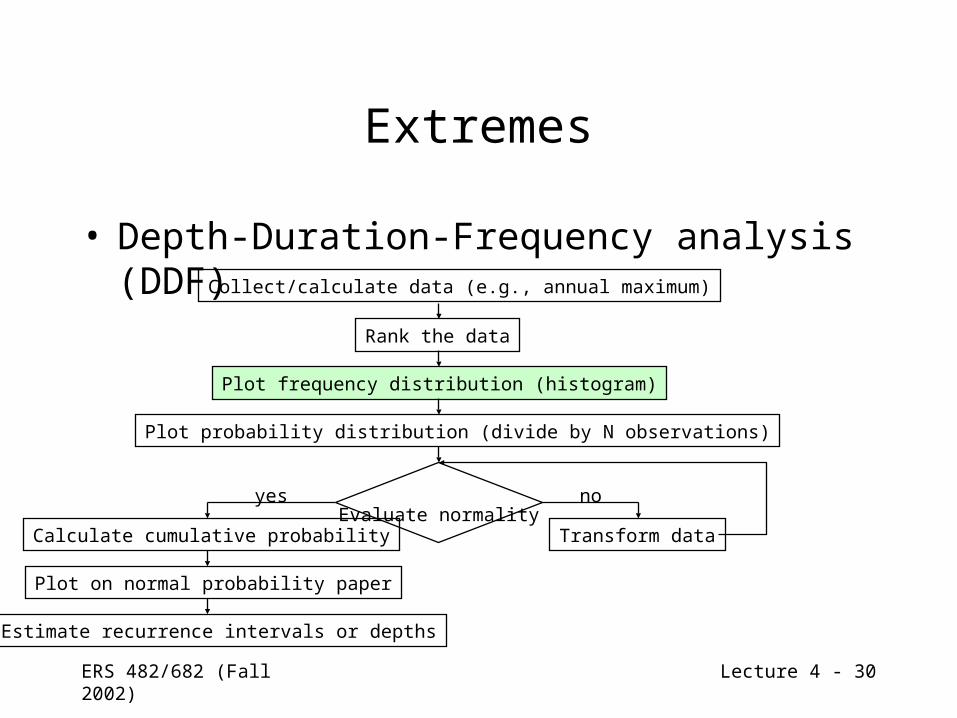
Extremes
• Depth-Duration-Frequency analysis (DDF) Collect/calculate data (e.g., annual maximum)
Rank the data
Plot frequency distribution (histogram)
Plot probability distribution (divide by N observations)
Evaluate normalityCalculate cumulative probability
Plot on normal probability paper
Estimate recurrence intervals or depths
Transform data
yes no
ERS 482/682 (Fall 2002) Lecture 4 - 31
Discrete vs. continuous data
• Discrete data can only take on discrete values within a range
• Continuous data can take on any value within a range
ERS 482/682 (Fall 2002) Lecture 4 - 32
Extremes
• Depth-Duration-Frequency analysis (DDF) Collect/calculate data (e.g., annual maximum)
Rank the data
Plot frequency distribution (histogram)
Plot probability distribution (divide by N observations)
Evaluate normalityCalculate cumulative probability
Plot on normal probability paper
Estimate recurrence intervals or depths
Transform data
yes no

ERS 482/682 (Fall 2002) Lecture 4 - 33
Extremes
• Depth-Duration-Frequency analysis (DDF) Collect/calculate data (e.g., annual maximum)
Rank the data
Plot frequency distribution (histogram)
Plot probability distribution (divide by N observations)
Evaluate normalityCalculate cumulative probability
Plot on normal probability paper
Estimate recurrence intervals or depths
Transform data
yes no
ERS 482/682 (Fall 2002) Lecture 4 - 34
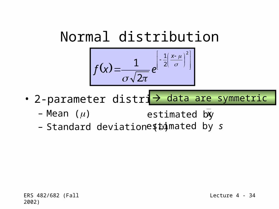
Normal distribution
• 2-parameter distribution:– Mean () – Standard deviation ()
xestimated byestimated by s
2
2
1
2
1
x
exf
data are symmetric
ERS 482/682 (Fall 2002) Lecture 4 - 35
Extremes
• Depth-Duration-Frequency analysis (DDF) Collect/calculate data (e.g., annual maximum)
Rank the data
Plot frequency distribution (histogram)
Plot probability distribution (divide by N observations)
Evaluate normalityCalculate cumulative probability
Plot on normal probability paper
Estimate recurrence intervals or depths
Transform data
yes no
ERS 482/682 (Fall 2002) Lecture 4 - 36
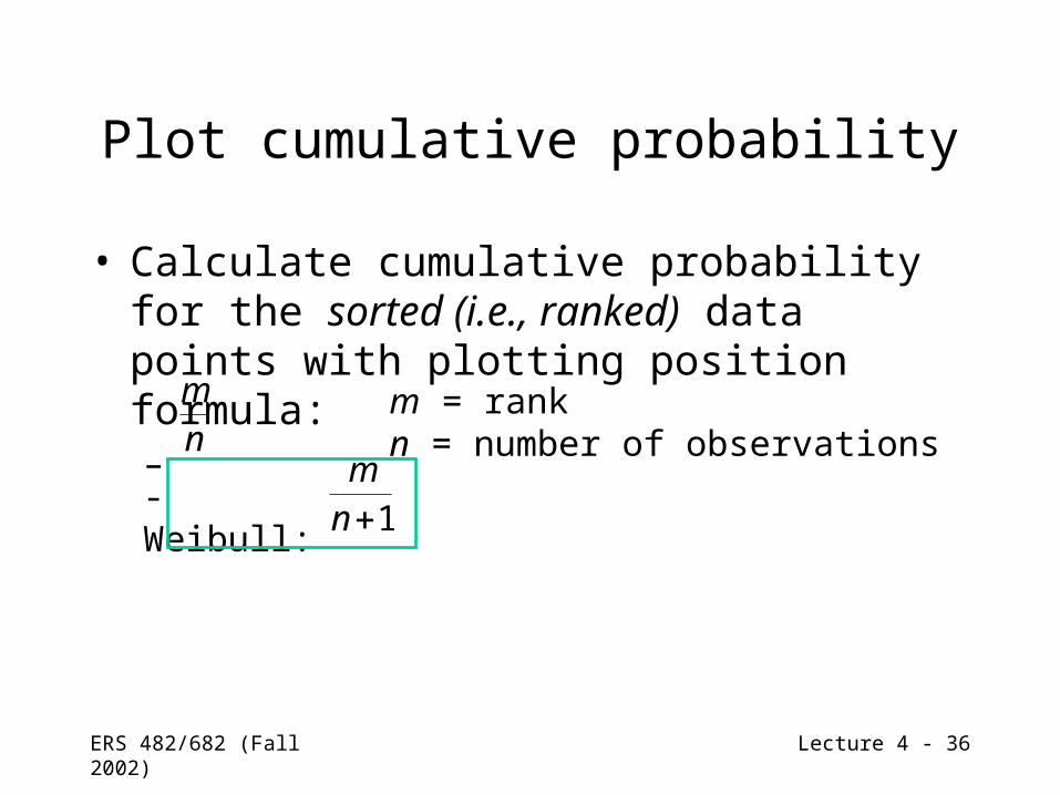
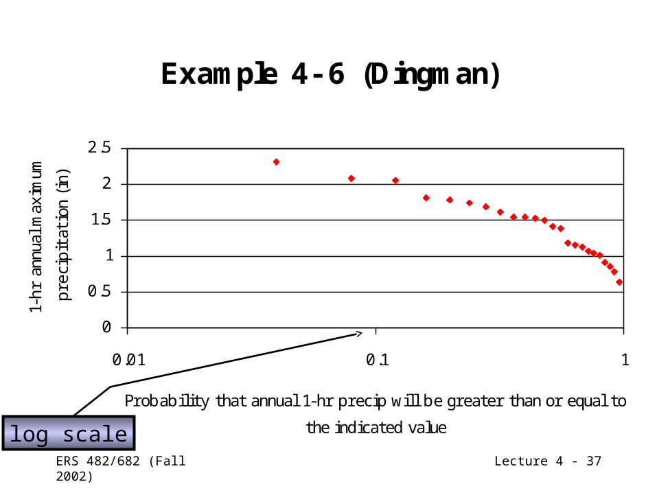
Plot cumulative probability
• Calculate cumulative probability for the sorted (i.e., ranked) data points with plotting position formula:– nm
1nm
- Weibull:
m = rankn = number of observations
ERS 482/682 (Fall 2002) Lecture 4 - 37
Example 4- 6 (Dingman)
0
0.5
1
1.5
2
2.5
0.01 0.1 1
Probability that annual 1-hr precip will be greater than or equal to
the indicated value
1-hr
ann
ual m
axim
um
prec
ipit
atio
n (i
n)
log scale
ERS 482/682 (Fall 2002) Lecture 4 - 38
Extremes
• Depth-Duration-Frequency analysis (DDF) Collect/calculate data (e.g., annual maximum)
Rank the data
Plot frequency distribution (histogram)
Plot probability distribution (divide by N observations)
Evaluate normalityCalculate cumulative probability
Plot on normal probability paper
Estimate recurrence intervals or depths
Transform data
yes no
ERS 482/682 (Fall 2002) Lecture 4 - 39
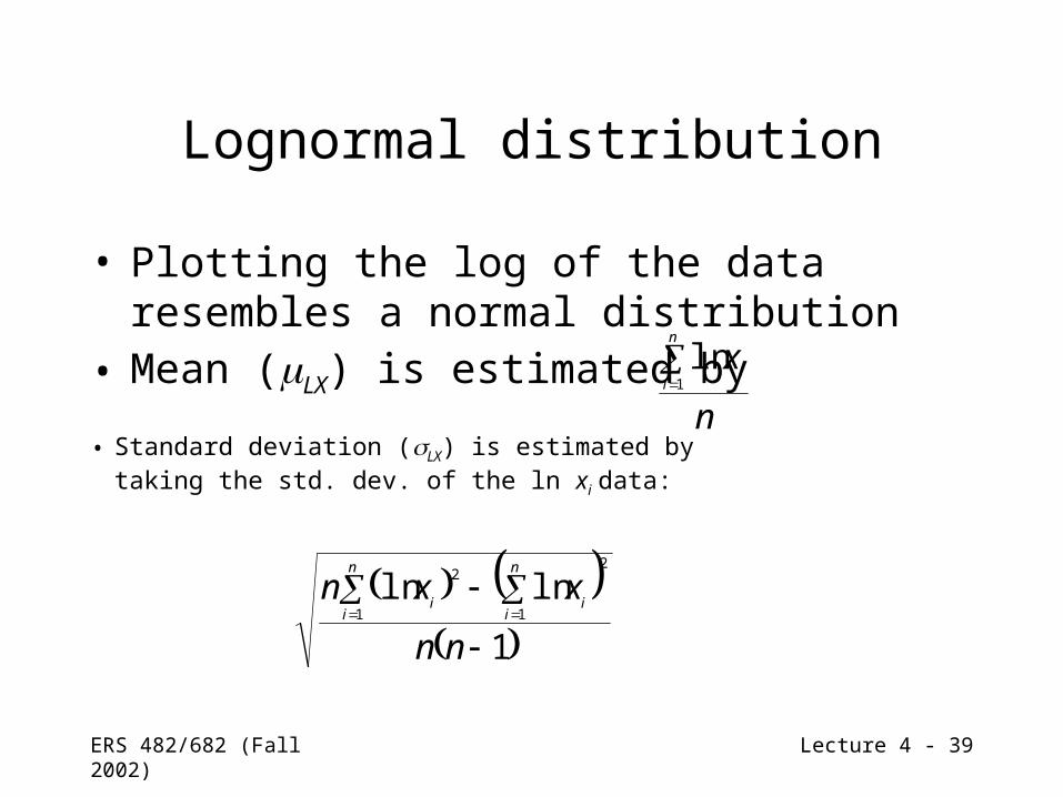
Lognormal distribution
• Plotting the log of the data resembles a normal distribution
n
xn
ii
1
ln• Mean (LX) is estimated by
• Standard deviation (LX) is estimated bytaking the std. dev. of the ln xi data:
1
lnln1
2
1
2
nn
xxnn
i
n
iii
ERS 482/682 (Fall 2002) Lecture 4 - 40
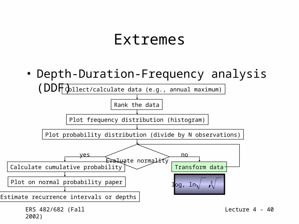
Extremes
• Depth-Duration-Frequency analysis (DDF) Collect/calculate data (e.g., annual maximum)
Rank the data
Plot frequency distribution (histogram)
Plot probability distribution (divide by N observations)
Evaluate normalityCalculate cumulative probability
Plot on normal probability paper
Estimate recurrence intervals or depths
Transform data
yes no
log, ln, 3,
ERS 482/682 (Fall 2002) Lecture 4 - 41
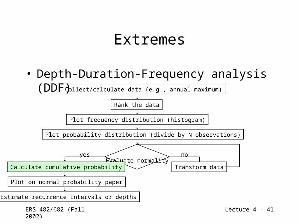
Extremes
• Depth-Duration-Frequency analysis (DDF) Collect/calculate data (e.g., annual maximum)
Rank the data
Plot frequency distribution (histogram)
Plot probability distribution (divide by N observations)
Evaluate normalityCalculate cumulative probability
Plot on normal probability paper
Estimate recurrence intervals or depths
Transform data
yes no
ERS 482/682 (Fall 2002) Lecture 4 - 42
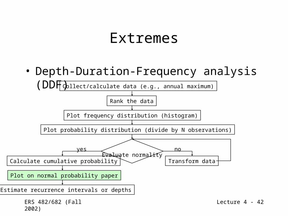
Extremes
• Depth-Duration-Frequency analysis (DDF) Collect/calculate data (e.g., annual maximum)
Rank the data
Plot frequency distribution (histogram)
Plot probability distribution (divide by N observations)
Evaluate normalityCalculate cumulative probability
Plot on normal probability paper
Estimate recurrence intervals or depths
Transform data
yes no
ERS 482/682 (Fall 2002) Lecture 4 - 43
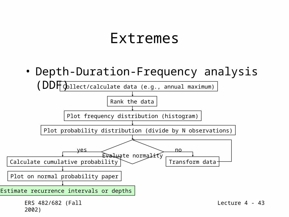
Extremes
• Depth-Duration-Frequency analysis (DDF) Collect/calculate data (e.g., annual maximum)
Rank the data
Plot frequency distribution (histogram)
Plot probability distribution (divide by N observations)
Evaluate normalityCalculate cumulative probability
Plot on normal probability paper
Estimate recurrence intervals or depths
Transform data
yes no
ERS 482/682 (Fall 2002) Lecture 4 - 44
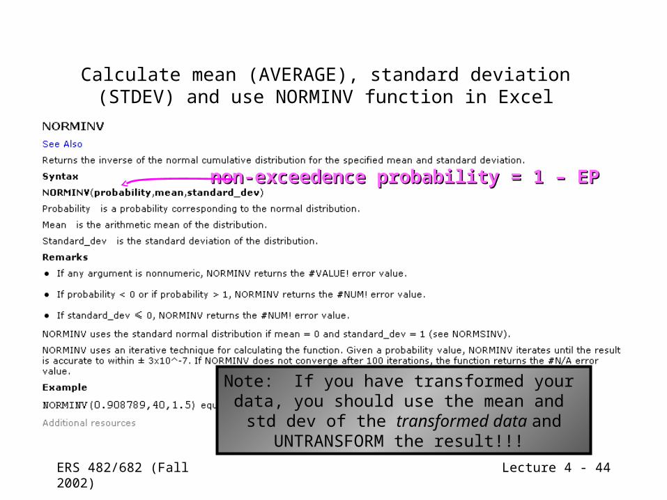
Calculate mean (AVERAGE), standard deviation (STDEV) and use NORMINV function in Excel
non-exceedence probability = 1 – EPnon-exceedence probability = 1 – EP
Note: If you have transformed your data, you should use the mean and std dev of the transformed data and
UNTRANSFORM the result!!!
ERS 482/682 (Fall 2002) Lecture 4 - 45
Extremes
• Depth-Duration-Frequency analysis (DDF)– Determine point rainfall depth for storm of
particular• Return period (e.g., 25-year, 100-year, etc.)• Duration (e.g., 1-hr, 2-hr, 6-hr, 24-hr, etc.)– Adjust point estimate to areal estimate• Equation 4-29 or Figure 4-52 or Figures 16.10 and
16.13 of Viessman and Lewis (1996)