Lecture 32: Security Vulnerabilities of Mobile … 32: Security Vulnerabilities of Mobile Devices...
91
Lecture 32: Security Vulnerabilities of Mobile Devices Lecture Notes on “Computer and Network Security” by Avi Kak ([email protected]) April 19, 2018 1:45pm c 2018 Avinash Kak, Purdue University Goals: • What makes mobile devices less vulnerable to malware — to the extent that is the case • Protection provided by sandboxing the apps • Security (or lack thereof) provided by over-the-air encryption for cellular communications with a Python implementation of A5/1 cipher • Side-channel attacks on specialized mobile devices • Examples of side-channel attacks: fault injection attacks and timing at- tacks • Python scripts for demonstrating fault injection and timing at- tacks • USB devices as a source of deadly malware • Mobile IP
Transcript of Lecture 32: Security Vulnerabilities of Mobile … 32: Security Vulnerabilities of Mobile Devices...

Lecture 32: Security Vulnerabilities of Mobile Devices
Lecture Notes on “Computer and Network Security”
by Avi Kak ([email protected])
April 19, 20181:45pm
c©2018 Avinash Kak, Purdue University
Goals:
• What makes mobile devices less vulnerable to malware — to the extent
that is the case
• Protection provided by sandboxing the apps
• Security (or lack thereof) provided by over-the-air encryption for cellular
communications with a Python implementation of A5/1 cipher
• Side-channel attacks on specialized mobile devices
• Examples of side-channel attacks: fault injection attacks and timing at-tacks
• Python scripts for demonstrating fault injection and timing at-
tacks
• USB devices as a source of deadly malware
• Mobile IP

CONTENTS
Section Title Page
32.1 Malware and Mobile Devices 3
32.2 The Good News is ... 9
32.3 Sandboxing the Apps 13
32.4 What About the Security of Over-the-Air 29Communications with Mobile Devices?
32.4.1 Python Implementation of A5/1 Cipher 36
32.5 Side-Channel Attacks on Specialized 43Mobile Devices
32.6 Fault Injection Attacks 46
32.6.1 Demonstration of Fault Injection with a 53Python script
32.7 Timing Attacks 58
32.7.1 A Python Script That Demonstrates How 66To Use Code Execution Time for Mountinga Timing Attack
32.8 USB Memory Sticks as a Source of 81Deadly Malware
32.9 Mobile IP 88
2
Computer and Network Security by Avi Kak Lecture 32
32.1: MALWARE AND MOBILE DEVICES
• Mobile devices — cellphones, smartphones, smartcards, tablets,
navigational devices, memory sticks, etc., — have now permeated
nearly all aspects of how we live on a day-to-day basis. While at
one time their primary function was only communications, now
they are used for just about everything: as cameras, as music
players, as news readers, for checking email, for web surfing, for
navigation, for banking, for connecting with friends through social
media, and, Ah!, not to be forgotten, as boarding passes when
traveling by air.
• A unanimous ruling by the Supreme Court of the United States
not too long ago is indicative of how integral and central such
devices have become to our lives. In a 9-0 decision on June 25,
2014, the justices ruled that police may not search a suspect’s cell-
phone without a warrant. Normally, police is allowed to search
your personal possessions — such as your wallet, briefcase, vehi-
cle, etc. — without a warrant if there is “probable cause” that a
crime was committed. Regarding cellphones, Chief Justice John
Roberts said: “They are such a pervasive and insistent part of
daily life that the proverbial visitor from Mars might conclude
they were an important feature of human anatomy.” Justice
3

Computer and Network Security by Avi Kak Lecture 32
Roberts also observed: “Modern cellphones, as a category, impli-
cate privacy concerns far beyond those implicated by the search
of a cigarette pack, a wallet, or a purse. Cell phones differ in
both a quantitative and a qualitative sense from other objects
that might be kept on an arrestee’s person.”
• The justices obviously based their decision on the fact that peo-
ple now routinely store private and sensitive information in their
mobile devices — the sort of information that you would have
stored securely at home in the years gone by.
• Given this modern reality, it is not surprising that folks who
engage in the production and propagation of malware are training
their guns increasingly on mobile devices.
• In a report on the security of mobile devices submitted to Congress,
the United States Government Accountability Office (GAO) stated
that the number of different malware variants aimed at smart-
phones had increased from 14,000 to 40,000 in just one year
(from July 2011 to May 2012). You can access this report at
http://www.gao.gov/assets/650/648519.pdf [The same report also mentions that the world-
wide sales of mobile devices increased from 300 million to 650 million in 2012. Now consider the fact
that over 1.5 billion smartphones (with a total sales value close to $500 billion) were sold in
2017. And that’s just the smartphones among all sorts of mobile devices. The numbers for 2017 are from
https://www.statista.com/topics/840/smartphones/]
4

Computer and Network Security by Avi Kak Lecture 32
• Mobile devices have become a magnet for malware producers
because they can be a source of sensitive information that an
attacker may be able to use for monetary gain, to seek political
advantage, to use as a means to break into a corporate network,
and so on.
• As you would expect, many of the attack methods on mobile
devices are the same as those on the more traditional computing
devices such as desktops, laptops, etc., — except for one very
important difference: Unless it is in a private network, a non-
mobile host is usually directly plugged into the internet where
it is constantly exposed to break-in attempts through software
that scans large segments of IP address blocks for discovering
vulnerable hosts. That is, in addition to facing targeted attacks
through social engineering and other means, a non-mobile host
connected to the internet also faces un-targeted attacks by cyber
criminals who simply want to discover hosts (regardless of where
they are) on which they can install their malware.
• On the other hand, mobile devices when they are plugged
into cellular networks can only be accessed by outsiders through
gateways that are tightly controlled by the cellphone companies.
[Consider the opposite situation of a mobile device being able to access the internet
directly through, say, a WiFi network. When on WiFi, the mobile device will be in
a private network (normally a class A or class C private network) behind a wireless
router/access-point. So the mobile device would not be exposed directly to IP address-
block scanning. However, now, a mobile device could be vulnerable to eaves-
5

Computer and Network Security by Avi Kak Lecture 32
dropping and man-in-the-middle attacks if, say, you are exchanging sensitive
information with a remote host in plain text. In the most common modes
of using a smartphone, though, you are unlikely to be a target of even such
attacks on account of the overall security provided by the servers. For exam-
ple, your smartphone will establish a secure link with a website like Amazon.com before
uploading your credit-card information to that website. As you know from Lecture 13,
your smartphone will accomplish that by downloading Amazon.com’s certificate, verify-
ing the certificate with the public key of the applicable root CA that is already stored
in your smartphone, and your smartphone and the remote website will then jointly
establish a session key for content encryption.]
• Therefore, it is unlikely that a mobile device you own is going to
get hit by random fly-by attack software.
• On account of the protection provided by (1) the cellular com-
pany gateways; (2) the protection made possible by encrypted
connections with servers that seek your private information; (3)
the protection provided by on-line app stores (like Google Play
and Apple’s App Store) through their vetting of the apps for se-
curity holes before making them available to you; and, finally, (4)
the protection provided by the fact that a mobile OS is likely to
run the apps in a sandbox; it is not surprising that malware in-
fection rates in smartphones are as low as mentioned in the next
section.
• However, the mobile devices are just as vulnerable to social
6

Computer and Network Security by Avi Kak Lecture 32
engineering attacks as the more traditional computing devices
such as desktops and laptops. (See Lecture 30 for Social En-
gineering attacks.) Of course, it goes without saying that if a
mobile device contains unpatched software with known vulner-
abilities, the device could be exploited through regular network
attacks that do not depend on social engineering.
• Additionally, a certain class of more specialized mobile devices
— smartcards in particular — may be vulnerable to attacks that
come under the category of side-channel attacks. [Smartcards have become
ubiquitous. They are now used for paying fare in public transportation systems, car theft protection (your
electronic car key), access control in buildings, etc.] These attacks are most effective
if an adversary can take physical control of a mobile device and
subject it to scrutiny that either treats it as a block box and ap-
plies different kinds of inputs to it, or, when possible, examines it
directly at the hardware/circuit level. Karsten Nohl gave a Black
Hat talk in 2008 that showed how he could break the encryption
in Mifare smartcards directly from the silicon. [A famous line from
that talk: “There are no secrets in silicon”] Check it out at:
https://www.blackhat.com/presentations/bh-jp-08/bh-jp-08-Nohl/BlackHat-Japan-08-Nohl-Secret-Algorithms-in-Hardware.pdf
• In the rest of this lecture, I’ll first review the concepts of sand-
boxing the apps since that adds significantly to the protection of
a mobile device against malicious apps.
• Next, I’ll review the A5/1 algorithm that has been widely de-
7

Computer and Network Security by Avi Kak Lecture 32
ployed around the world for encrypting over-the-air voice and
SMS data in GSM (2G) cellphone networks. This algorithm is one
of the best case studies in what can happen when people decide
to create security by obscurity. This algorithm was kept secret
for several years by cellphone operators. As is almost always the
case with such things, eventually the algorithm was leaked out.
As soon as the algorithm made its way into the public domain,
it was shown to possess practically no security.
• Then I’ll will present what is meant by side-channel attacks.
As mentioned previously in this section, specialized mobile de-
vices such as smartcards are particularly vulnerable to these at-
tacks. In order to lend further clarity to how one can construct
such attacks, I’ll provide my Python implementations for some
of the more common forms of such attacks.
• Finally, I’ll go over a topic that has been much in the news lately:
the ease with which malware infections can be spread with USB
devices such as memory sticks and why such infections cannot be
detected by common anti-virus tools.
8
Computer and Network Security by Avi Kak Lecture 32
32.2: THE GOOD NEWS IS ...
• As was mentioned toward the end of the previous section, mobile
devices — especially of the smartphone variety — benefit from
multiple layers of protection. These are:
– For the most part, individual smartphones can only be accessed through
the gateways controlled by the cellular network companies;
– When engaged in e-commerce interactions and regardless of whether
a smartphone is communicating directly over a cellular network orthrough WiFi, the fact that a smartphone and the server create an
encrypted session before any sensitive information is exchanged be-tween the two (in accordance with client-server interactions described
in Lecture 13);
– The app stores (Google Play, Apple’s App Store, Windows PhoneStore) scan and analyze the apps for malware before making themavailable to customers;
– The fact that apps are typically run by the mobile OS in a sandbox.
This is certainly true of the Android OS for the Android devices; iOSfor all mobile devices by Apple and that includes various versions
of iPhones, iPods, and iPads; and the Windows Phone OS for theWindows based mobile devices.
9

Computer and Network Security by Avi Kak Lecture 32
• Despite these layers of protection, the security of a smartphone
can easily be compromised by: (1) man-in-the-middle attacks
when the device is plugged into an unlocked WiFi network (es-
pecially if the user is sending or receiving sensitive information
in plaintext); and (2) a user visiting a website that tricks or lures
the user into downloading a document that either is malware or
contains malware. But then these forms of vulnerability apply
just as much to non-mobile computing devices such as desktops
and laptops.
• Nonetheless, it remains that the four layers of security mentioned
on the previous page make it less likely that your smartphone
contains malware. This conclusion is borne out by the report
“Android Security, 2017 Year in Review” just released by Google
that you’ll find at the following URL:
https://source.android.com/security/reports/Google_Android_Security_2017_Report_Final.pdf
• The Android security report says:
“In 2016, the annual probability that a user downloaded a Poten-tially Harmful Applications (PHA) from Google Play was .04%
and we reduced that by 50% in 2017 for an annual average of.02%. In 2017, downloading a PHA from Google Play was
less likely than the odds of an asteroid hitting the earth.”
• While it is comforting to know that overall the probability of your
Android device becoming infected with malware is low, it would
10

Computer and Network Security by Avi Kak Lecture 32
still be highly educational for the reader to go through the last
eight pages of the Android security report and read about the
different malware families that are currently making the rounds
in the Android ecosystem.
• One of the nastier examples of this malware was much in the
new last year: Spying on Android users through otherwise be-
nign apps that used presumably legitimate ad network SDK to
dish out the ads. As you surely know already, SDK stands for
“Software Development Kit” and an ad network SDK is a soft-
ware package, made available by an ad network organization, that
app developers incorporate in their apps. Subsequently, the ad
network in question can decide what ads to show to the Android
device users and track the effectiveness of those ads in generating
revenue that is shared by the ad network organization and the
advertisers.
• Last year, Lookout, a security company (https://www.lookout.com) spe-
cializing in issues related to mobile devices, discovered that the ad
network SDK made available by an ad network company called
Igexin was downloading encrypted malicious plugins into the An-
droid devices from the Igexin servers and uploading to the servers
the users’ private data. What is most important here is that
when these apps were submitted to Google Play, there was no
hint of malware in them. Presumably, the app developers them-
selves were completely in the dark about how their apps would
be misused by the ad network organization after the apps had
11

Computer and Network Security by Avi Kak Lecture 32
been accepted by Google Play.
• In their report, Lookout mentions that the apps containing the
affected SDK were downloaded over 100 million times across
the Android ecosystem.
12

Computer and Network Security by Avi Kak Lecture 32
32.3: SANDBOXING THE APPS
• A great deal of the security you get with mobile devices such as
smartphones is owing to the fact that the third-party software
(the apps) is executed in a sandbox. This is true for all major
mobile operating systems today, such as the Android OS, iOS,
Windows Phone OS, etc.
• In general, each app is run as a separate process in its own sand-
box.
• Sandboxing means isolating the app processes from one another,
on the one hand, and from the system resources, on the other.
Sandboxing also requires putting in place a permissions frame-
work that tightly regulates as to which other apps get access to
the data produced by any given app. [Sandboxing is now also widely used for
desktop/laptop applications. The web browser on your desktop/laptop is most likely being run in a sandbox.
That way, any data downloaded/created by say a plug-in like Adobe Flash or Microsoft Silverlight is unlikely
to corrupt your other files even when the downloaded data contains malware. Sandboxes are now also used by
document readers for PDF and other formats so that any malware macros in those documents do not harm
the other files.]
13

Computer and Network Security by Avi Kak Lecture 32
• The rest of this section focuses primarily on how Android isolates
a process by running it in a sandbox. However, before talking
about sandboxing in Android, let’s quickly review some of the
highlights of the Android OS since it is the OS that demands
that each app run in its own sandbox.
• I suppose you already know that Android was born from Linux.
The very first release of Android was based on Version 2.6.25 of
the Linux kernel. More recent versions of Android are based on
Versions 3.4, 3.8 and 3.10 of the Linux kernel, depending on the
unerlying hardware platform. (As of mid April 2018, the latest
stable version of the Linux kernel was 4.16.2 according to the
information posted at the http://www.kernel.org website.) [If you are
using your knowledge of Linux as a springboard to learn about Android, a good place to visit to learn about the
features that are unique to Android is http://elinux.org/Android_Kernel_Features . To summarize some of
the main differences: (1) One significant difference relates to how the interprocess communications is carried
out in Android. (2) Android’s power management primitive known as “wakelock” that an app can use to
keep the CPU humming at its normal frequency and the screen on even in the absence of any user interaction.
The normal mode of smartphone operation requires that the phone go into deep sleep (by turning off the
screen and reducing the frequency of the CPU in order to conserve power) when there is no user interaction.
However, that does not work for, say, a Facebook app that may need to check on events every few minutes.
Those sorts of apps can acquire a wakelock to keep the CPU running at its normal frequency and, if needed,
to turn on the screen when a new event of interest to the smartphone owner is detected. (Since the Facebook
app’s need to acquire the wakelock every few minutes can put a drain on your battery, some Android users
install a free root app called Greenify to first get a sense of how much battery is consumed by such an app
and to then better control its need to wake up frequently.) (3) Android’s memory allocation functions. (4)
And so on. In addition to these differences between Linux and Android, note also that the Android OS must
14

Computer and Network Security by Avi Kak Lecture 32
work with several different types of sensors and hardware components that a desktop/laptop OS need not
bother with. We are talking about sensors and hardware components such as the touchscreen, cameras, audio
components, orientation sensors, accelerometers, gyroscopes, etc. Finally, note that Android was originally
developed for the ARM architecture. However, it is now also supported for the x86 and the MIPS processor
architectures.] Despite the differences between Linux and Android,
the Linux Foundation and many others consider Android to be a
Linux distribution (even though it does not come with the Gnu
C libraries, etc. Android comes with its own C library that has
a smaller memory footprint; it is called Bionic).
• As already mentioned, every Android app — written in Java —
is run in a sandbox as a separate process. [More precisely speaking, a separate
process is created for a digitally signed Linux user ID. If there exist multiple apps that are associated with
the same Linux user ID, they can all be run in the same Linux process. Here is a good tutorial on how
you go about creating public and private keys for digitally signing an Android app that you have created:
http://www.ibm.com/developerworks/library/x-androidsecurity/] When you download
a new app or update one of the apps already in your device, it
is this sandboxing feature that causes your smartphone to ask
you whether the app is allowed to access the data produced by
other programs and various components of your smartphone —
these would be the location information, the camera, the logs,
the bookmarks, etc.
• By default, an app runs with no permissions assigned to it. When
an app requests access to the data produced by another app, it
is subject to the rules declared in the latter’s manifest file.
15

Computer and Network Security by Avi Kak Lecture 32
• Sandboxing ensures that, in general, any files created by an app
can only be read by that app. Android does give app developers
facilities for creating more globally accessible files through modes
named MODE WORLD WRITABLE and MODE WORLD READABLE. Apps using
these read/write modes are subject to greater scrutiny from a
security standpoint.
• For greater control over what other app processes can access the
data created by your own app, instead of using the two read/write
modes mentioned in the previous bullet, your app can place
its data in an object that is subclassed from the Android Java
class ContentProvider and specify its android:exported, android:
protectionLevel, and other attributes. [In most cases, a ContentProvider stores
its information in an SQlite database, which as its name implies is an SQL database for storing structured
information. An app requesting information from such a database must first create a client by subclassing from
the Java class ContentResolver.]
• In Linux systems, the two most widely deployed techniques for
sandboxing a process are SELinux and AppArmor. SELinux —
the name is a shorthand for “Security Enhanced Linux” — is
a Linux kernel module that makes it possible for the operating
system to exercise fine-grained access control with regard to the
resource requests by running programs.
• Both SELinux and AppArmor are based on the LSM (Linux Se-
curity Modules) API for enforcing what is known as Mandatory
16

Computer and Network Security by Avi Kak Lecture 32
Access Control (MAC). MAC is meant specifically for operating
systems to place constraints on the resources that can be accessed
by running programs. By resources, we mean files, directories,
ports, communication interfaces, etc.
• Perhaps the most significant difference between SELinux and Ap-
pArmor is that the former is based on context labels that are
associated with all the files, the interfaces, the system resources,
etc., and the latter is based on the pathnames to the same. [By
default, Ubuntu installs Linux with AppArmor. However, you can yourself install the SELinux kernel patch
through the Synaptic Package Manager. Keep in mind, though, when you install SELinux, the AppArmor pack-
age will be automatically uninstalled. About comparing SELinux with AppArmor, there are many developers
out there who prefer the latter because they consider the SELinux policy rules for isolating the processes to be
much too complex for manual generation. While there do exist tools that can generate the rules for you, the
complexity of the rules makes it difficult to verify them, according to these developers. On the other hand, the
AppArmor rules are relatively simple, can be expressed manually, and are therefore more amenable to human
validation. However, the access control you can achieve with AppArmor is not as fine grained as what you can
get with SELinux.] The following three sources provide a comparative
assessment of SELinux and AppArmor for isolating the processes
running in your computer:
http://elinux.org/images/3/39/SecureOS_nakamura.pdf
http://researchrepository.murdoch.edu.au/6177/1/empowering_end_users.pdf
https://www.suse.com/support/security/apparmor/features/selinux_comparison.html
• The Mandatory Access Control (MAC) used by Android to iso-
late a process by running it in a sandbox is based on SELinux. [This
17

Computer and Network Security by Avi Kak Lecture 32
is true for versions 4.3 and higher of Android. I believe the latest version of Android
is 8.1 Oreo.] For that reason, the rest of this section focuses on
SELinux.
• A good starting point for understanding the access control made
possible by SELinux is what you get with a standard distribution
of Linux. The standard distribution regulates access on the basis
of the privileges associated with a running program. In general,
if a program runs with superuser privileges (that is, privileges
associated with user ID 0), it can bypass all security restrictions.
That is, such a program has no constraints regarding what files,
interfaces, interprocess communications, and so on, it can access.
(Just imagine a rogue program in your machine that has managed
to guess your root password.) [In case you happen to be thinking of access privileges in
Windows platforms, the accounts SYSTEM and ADMINISTRATOR have privileges similar to those of root
in Unix/Linux systems.] The access control in a standard distribution of
Linux is referred to as the Linux Discretionary Access Control
(DAC).
• SELinux, on the other hand, associates a context label with every
file, directory, user account, process, etc., in your computer. A
context label consists of four colon separated parts (with the last
part being optional):
user : role : type : level
You can see the context label associated with a file or a directory
by executing the command ‘ls -Z filename’. For example, when
18
Computer and Network Security by Avi Kak Lecture 32
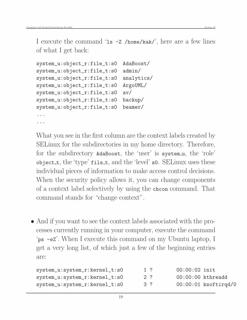
I execute the command ‘ls -Z /home/kak/’, here are a few lines
of what I get back:
system_u:object_r:file_t:s0 AdaBoost/
system_u:object_r:file_t:s0 admin/
system_u:object_r:file_t:s0 analytics/
system_u:object_r:file_t:s0 ArgoUML/
system_u:object_r:file_t:s0 av/
system_u:object_r:file_t:s0 backup/
system_u:object_r:file_t:s0 beamer/
...
...
What you see in the first column are the context labels created by
SELinux for the subdirectories in my home directory. Therefore,
for the subdirectory AdaBoost, the ‘user’ is system u, the ‘role’
object t, the ‘type’ file t, and the ‘level’ s0. SELinux uses these
individual pieces of information to make access control decisions.
When the security policy allows it, you can change components
of a context label selectively by using the chcon command. That
command stands for “change context”.
• And if you want to see the context labels associated with the pro-
cesses currently running in your computer, execute the command
‘ps -eZ’. When I execute this command on my Ubuntu laptop, I
get a very long list, of which just a few of the beginning entries
are:
system_u:system_r:kernel_t:s0 1 ? 00:00:02 init
system_u:system_r:kernel_t:s0 2 ? 00:00:00 kthreadd
system_u:system_r:kernel_t:s0 3 ? 00:00:01 ksoftirqd/0
19

Computer and Network Security by Avi Kak Lecture 32
system_u:system_r:kernel_t:s0 5 ? 00:00:00 kworker/0:0H
system_u:system_r:kernel_t:s0 7 ? 00:10:26 rcu_sched
system_u:system_r:kernel_t:s0 8 ? 00:05:49 rcuos/0
system_u:system_r:kernel_t:s0 9 ? 00:03:22 rcuos/1
...
...
...
• As you can imagine, when you associate with every entity in your
computer a context label of the sort shown above, you can set
up a fine-grained access control policy by placing constraints on
which resource a user (in the sense used in the context labels) in
a given role and of a certain given type and level is allowed to
access taking into account the resource’s own context label. You
can now create a Role-Based Access Control (RBAC) policy, or
a Type Enforcement (TE) policy, and, if SELinux specifies the
optional ‘level’ field in the context labels, a Multi-Level Security
(MLS) policy. In addition, you can set up a Multi-Category
Security (MCS) policy — we will talk about that later.
• To show a simple example of type enforcement from the SELinux
FAQ, assume that all the files in a user account are given the type
label user home t. And assume that the Firefox browser running
in your machine is given the type label firefox t. The following
access control declaration
allow firefox_t user_home_t : file { read write };
will then ensure that the browser has only read and write permis-
20

Computer and Network Security by Avi Kak Lecture 32
sions with respect to user files — even if the browser is being run
by someone with root privileges. [You can see why some people think of SELinux as a
firewall between programs. Ordinarily, as you saw in Lecture 18, a firewall regulates traffic between a computer
and the rest of the network.]
• In order to make it easier to create the access control policies for
a new application, SELinux gives you a Reference Policy that can
be modified as needed. A company named Tresys Technologies
updates the Reference Policy on the basis of the user feedback sent
to the Policy Project mailing list at GitHub. This reference policy
is typically customized by the provider of your Linux platform.
• In order to become more familiar with SELinux, you can down-
load and install SELinux in a Ubuntu machine through your
Synaptic Package Manager. [Or you can do ‘sudo apt-get remove apparmor’ followed
by ‘sudo apt-get install selinux’] Make sure you choose the meta-package
selinux and not the package selinux-basics. SELinux becomes
operational (although not enabled) just by installing it. Note
that with Ubuntu, the reference policy you get is stored in the
file /etc/selinux/ubuntu/policy/policy29.
• After you have installed SELinux as described above, you will
need to reboot the machine in order to enable SELinux. [During this
reboot, all of the files on the disk will acquire context labels in accordance with the explanation presented earlier
in this section.] Subsequently, if you execute a command like ‘sestatus’
(you don’t have to be root to run this command), you’ll see the
21

Computer and Network Security by Avi Kak Lecture 32
following output returned by SELinux:
SELinux status: enabled
SELinuxfs mount: /sys/fs/selinux
SELinux root directory: /etc/selinux
Loaded policy name: ubuntu
Current mode: permissive
Mode from config file: permissive
Policy MLS status: enabled
Policy deny_unknown status: allowed
Max kernel policy version: 28
If you now execute the command ‘sudo setenforce 1’, you’ll see
the same output as shown above, but with the line ‘Current mode:
permissive’ changed to ‘Current mode: enforcing’.
• If you want to see a listing of all the SELinux users, you can
enter the command ‘seinfo -u’. When I run this command on
my Ubuntu laptop, I get
Users: 6
sysadm_u
system_u
root
staff_u
user_u
unconfined_u
And if I execute the command ‘seinfo -r’ to see all of the roles
used in the context labels, I get back
22
Computer and Network Security by Avi Kak Lecture 32
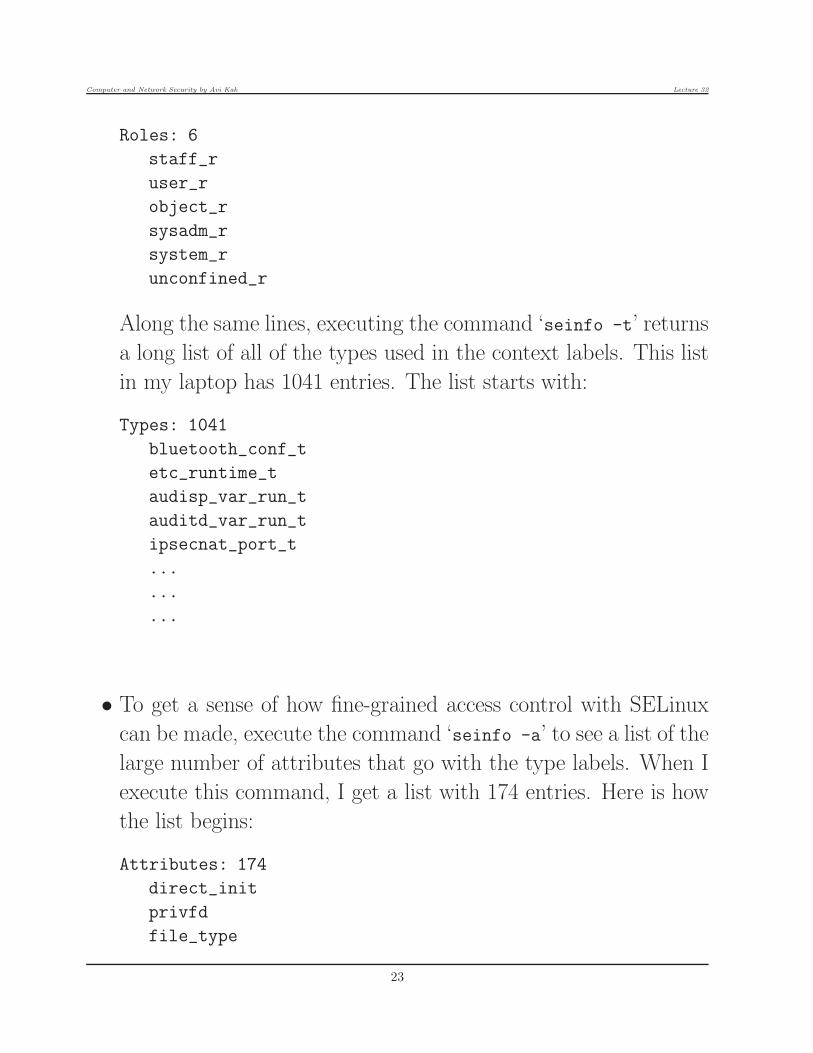
Roles: 6
staff_r
user_r
object_r
sysadm_r
system_r
unconfined_r
Along the same lines, executing the command ‘seinfo -t’ returns
a long list of all of the types used in the context labels. This list
in my laptop has 1041 entries. The list starts with:
Types: 1041
bluetooth_conf_t
etc_runtime_t
audisp_var_run_t
auditd_var_run_t
ipsecnat_port_t
...
...
...
• To get a sense of how fine-grained access control with SELinux
can be made, execute the command ‘seinfo -a’ to see a list of the
large number of attributes that go with the type labels. When I
execute this command, I get a list with 174 entries. Here is how
the list begins:
Attributes: 174
direct_init
privfd
file_type
23

Computer and Network Security by Avi Kak Lecture 32
mlsnetinbound
can_setenforce
exec_type
xproperty_type
dbusd_unconfined
kern_unconfined
mlsxwinwritecolormap
node_type
packet_type
proc_type
port_type
...
...
...
• In case you are curious, you can see the context label assigned to
your account name by entering the usual ‘id’ command. Prior to
installing SELinux, this command just returns the user ID and
group ID associated with your account. However, after having
installed SELinux, I get back the following (all in one line):
uid=1001(kak) gid=1001(kak) groups=1001(kak),4(adm),7(lp),27(sudo),109(lpadmin),124(sambashare)
context=system_u:system_r:kernel_t:s0
What you see at the end is the context label associated with my
account. If I just wanted to see the context label, I can execute
the command ‘id -Z’. Running this command yields
system_u:system_r:kernel_t:s0
24

Computer and Network Security by Avi Kak Lecture 32
which says that I am a system u user (presumably because of my
sudo privileges), that my role is system r, that the type label
associated with me is kernel t, and that my level is s0.
• Remember the following six SELinux users returned by the com-
mand ‘seinfo -u’: sysadm u, system u, root, staff u, user u, and
unconfined u. Suppose we want to find out what different possi-
ble roles can be played by each of these users, we can execute the
command ‘sudo semanage user -l’. This command returns:
Labeling MLS/ MLS/
SELinux User Prefix MCS Level MCS Range SELinux Roles
root user s0 s0-s0:c0.c255 staff_r sysadm_r system_r
staff_u user s0 s0-s0:c0.c255 staff_r sysadm_r
sysadm_u user s0 s0-s0:c0.c255 sysadm_r
system_u user s0 s0-s0:c0.c255 system_r
unconfined_u user s0 s0-s0:c0.c255 system_r unconfined_r
user_u user s0 s0 user_r
This display shows that a ‘root’ user in my laptop is allowed to
acquire any of the three roles: staff r, sysadm r, and system r.
However, since as ’kak’ I am a system u user, the only role I am
allowed is system r.
• Let’s now talk about the fourth column in the tabular presenta-
tion returned by the command ‘sudo semanage user -l’. This is
the column with the heading “MLS/MCS Range”. Each entry in
this column consists of two parts that are separated by a colon.
What is to the left of the colon is the range of levels that is al-
lowed for each SELinux user (where, again, by ’user’ we mean
25

Computer and Network Security by Avi Kak Lecture 32
one of the six user labels that SELinux understands). As you will
recall, earlier in this section we talked about MLS standing for
Multi-Level Security that is made possible by the level field in the
context labels. What is displayed on the right of the colon — it
is important to the implementation of an MCS (Multi-Category
Security) access control policy mentioned earlier — is the range of
categories allowed for each SELinux user. You can, for example,
associate a set of different categories with each file in a directory.
A user will be able to access a file in that directory only if
the user belongs to all of the categories specified for that file.
The declaration syntax ‘c0.c255’ is a shorthand for categories c0
through c255. When MCS based access control is used, it comes
subsequent to the access control stipulated by LDAC, and the
access constraints created through role-based, type-based, and
level-based access control enforcement. So MCS can only further
constrain what resources can be accessed on a computer. [As men-
tioned earlier in this section, the access control made available by a standard distribution of Linux is referred
to as Linux Discretionary Access Control (DAC).]
• In case you need to, you can disable SELinux with a command
like
sudo setenforce 0
and re-enable it with
sudo setenforce 1
As mentioned earlier, you can check the status of SELinux run-
ning on our machine by
26

Computer and Network Security by Avi Kak Lecture 32
sestatus
If it says “enforcing,” that means that SELinux is providing pro-
tection. To completely disable the SELinux install in your ma-
chine, change the SELINUX variable in the /etc/selinux/config
file to read
SELINUX=disabled
• Should it happen that you run into some sort of a jam after
installing SELinux in a host, perhaps you could try executing
the command ‘sudo setenforce 0’ in that host in order to place
SELinux in a permissive mode. To elaborate with an example,
let’s say you try to scp a file into a SELinux enabled host as a user
named ‘xxxx’ (assuming that xxxx has login privileges at the host)
and it doesn’t work. You check the ‘/var/log/auth.log’ file in the
host and you see there the error message “failed to get default SELinux security
context for xxxx (in enforcing mode)”. In order to solve this problem, you’d need
to fix the context label associated with the user ‘xxxx’. Barring
that, you can also momentarily place the host in a permissive
mode through the command ‘sudo setenforce 0’ and get the job
done.
• What is achieved in Linux with MAC is achieved in Windows
systems with Mandatory Integrity Control (MIC) that associates
one of the following five Integrity Levels (IL) with processes: Low,
Medium, High, System, and Trusted Installer.
27

Computer and Network Security by Avi Kak Lecture 32
• While we achieve significant security by sandboxing the apps,
one cannot be lulled into thinking that that’s is the answer to
all systems related vulnerabilities in computing devices. When
it comes to systems related issues in computer security, here is
some food for thought: Is it possible that your OS bootstrap
loader (such as the GRUB bootloader) could be used by a rogue
program to download a corrupted OS kernel? Is it possible that
the /sbin/init file (that is used to launch the init process from
which all other processes are spawned in Unix/Linux platforms)
could itself be replaced by a corrupted version? And what about
an adversary exploiting the ptrace tools that is normally used
in Linux by one process to observe and control the execution of
another process?
28

Computer and Network Security by Avi Kak Lecture 32
32.4: WHAT ABOUT THE SECURITY OFOVER-THE-AIR COMMUNICATIONS
WITH MOBILE DEVICES?
• Even if we were to think that our smartphones are free of malware,
what would that imply with respect to the ability of the devices
to engage in secure voice and data communications with the
base stations of cellular operators? It is this question that I’ll
briefly address in this section.
• The answer to the question posed above depends on which genera-
tion of cellphone technology you are talking about. As you know,
we now have 2G (GSM), 3G (UMTS), 4G (LTE, ITU), and now
5G wireless standards for cellphone communications. The algo-
rithms that are used for encrypting over-the-air voice and data
communications with these different standards are referred to as
the A5 series of algorithms. The algorithm that is used for en-
crypting voice and SMS in the 2G standard (which, by the way,
still dominates in most geographies around the world) is the A5/1
stream cipher. A5/2, a weaker version of A5/1 created to meet
certain export restrictions of about a decade ago, turned out to
be an extremely weak cipher and has been discontinued. A5/3
and A5/4 are meant for 3G and 4G wireless technologies. [The GSM
29

Computer and Network Security by Avi Kak Lecture 32
standard defines a set of algorithms for encryption and authentication services. These algorithms are named
‘Ax’ where ‘x’ in an integer that indicates the function of the algorithm. For example, a base station can call
on the A3 algorithm to authenticate a mobile device. The A5 algorithm provides the encryption/decryption
services. The algorithm A8 is used to generate a 64 bit session key. An algorithm with the name COMP128
combines the functionality of A3 and A8.]
• Both A5/3 and A5/4 are based on the KASUMI block cipher,
which in turn is based on a block cipher called MISTY1 devel-
oped by Mitsubishi. The KASUMI cipher is used in the Output
Feedback Mode that we talked about in Lecture 9, which gener-
ates a bitstream in multiples of 64 bits. Regarding KASUMI, it
is a 64-bit block cipher with a Feistel structure (that you learned
in Lecture 3) with eight rounds. KASUMI needs a 128-bit en-
cryption key.
• The rest of this section, and the subsection that follows, focuses
on the A5/1 cipher that is used widely in 2G cellular networks. It
is now well known that this cipher provides essentially no security
because of the speed with which it can be cracked using ordinary
computing hardware.
• What makes A5/1 interesting is that it is a great case study in
how things can go wrong when you believe in security through
obscurity. As I mentioned in Section 32.1, this algorithm was
kept secret for several years by the cellphone operators. But,
eventually, it was leaked out and found to provide virtually no
30
Computer and Network Security by Avi Kak Lecture 32
security with regard to the privacy of voice data and SMS mes-
sages.
• A5/1 is bit-level stream cipher with a 64-bit encryption key. The
encryption key is created for each session from a master key that
is shared by the cellphone operator (with which the phone is
registered) and the SIM card in the phone. When a base station
(which may belong to some other cellphone operator) needs a
session key, it fetches it from the cellphone operator that holds
the master key.
• GSM transmissions are bursty. Time division multiplexing is used
to quickly transmit a collected stream of bits that need to be sent
over a given communication link between the base station and a
phone. A single burst in each direction consist of 114 bits of 4.615
milliseconds duration.
• The purpose of A5/1 is to produce two pseudorandom 114-bit
streams — called the keystreams — one for the uplink and the
other for the downlink. The 114-bit data in each direction is
XORed with the keystream. The destination can recover the
original data by XORing the received bit stream with the same
keystream.
• In addition to the 64-bit key, the encryption of each 114-bit
stream is also controlled by a 22-bit frame number which is always
31

Computer and Network Security by Avi Kak Lecture 32
publicly known.
• A5/1 works off three LFSRs (Linear Feedback Shift Register),
designated R1, R2, and R3, of sizes 19, 22, and 23 bits, as shown
in Figure 1. Each shift register is initialized with the 64-bit en-
cryption key and the 22-bit frame number in the manner illus-
trated by the Python code in the next subsection.
• Each shift register has what is known as a clocking bit — for
each register it’s marked with a red box in Figure 1. As you can
tell from the figure, for R1, the clocking bit is at index 8, and
for both R2 and R3 at index 10. During the production of the
keystream, the clocking bits are used to decide whether or not to
clock a shift register. [Pay close attention to the distinction between the clocking bit, of which
there is ONLY ONE in each shift register, and the feedback bits, of which there are SEVERAL in each shift
register, as shown in Figure 1.]
• Clocking a shift register involves the following operations: (1)
You record the bits at the feedback taps in the register; (2) You
shift the register by one bit position towards the MSB (which is at the
right end of the shift registers, the end with the highest indexed bit position); and (3) You set
the value of the LSB to an XOR of the feedback bits. When
you are first initializing a register with the encryption key, you
add a fourth step, which is to XOR the LSB with the key bit
corresponding to that clock tick, etc.
32

Computer and Network Security by Avi Kak Lecture 32
0 18
0 21
1
1
220 1
8
10
10
Register R1
Register R2
Register R3
Clocking Control
OutputKeystream
13 1617
20
20 217
Figure 1: This figure shows how three Linear Feedback Shift
Registers are used in the A5/1 algorithm for encrypting
voice and SMS in 2G cellular networks. (This figure is from Lecture 32
of “Lecture Notes on Computer and Network Security” by Avi Kak)
33

Computer and Network Security by Avi Kak Lecture 32
• After the shift registers have been initialized, you produce a
keystream by doing the following at each clock tick:
– You take a majority vote of the clocking bits in the three
registers R1, R2, and R3. Majority voting means that you
find out whether at least two of the three are either 0’s or 1’s.
– You only clock those registers whose clocking bits are in agree-
ment with the majority bit.
– You take the XOR of the MSB’s of the three registers and
that becomes the output bit.
• The next subsection presents a Python implementation of this
logic to remove any ambiguities about the various steps outlined
above.
• A5/1 has been the subject of cryptanalysis by several researchers.
The most recent attack on A5/1, by Karsten Nohl, was presented
at the 2010 Black Hat conference. The PDF of the paper is
available at:
https://srlabs.de/blog/wp-content/uploads/2010/07/Attacking.Phone_.Privacy_Karsten.Nohl_1.pdf
Here is a quote from Karsten Nohl’s paper:
34

Computer and Network Security by Avi Kak Lecture 32
“..... A5/1 can be broken in seconds with 2TB of fast storage and two graph-ics cards. The attack combines several time-memory trade-off techniques andexploits the relatively small effective key size of 61 bits”
Nohl has demonstrated that a rainbow table attack can be mounted
successfully on A5/1. You learned about rainbow tables in Lec-
ture 24.
• Another interesting (but more theoretical) paper about mount-
ing attacks on A5/1 is “Cryptanalysis of the A5/1 GSM Stream
Cipher” by Eli Biham and Orr Dunkelman that appeared in
Progress in Cryptology – INDOCRYPT, 2000. Another impor-
tant publication that talks about cryptanalysis of A5 ciphers
is “Instant Ciphertext-Only Cryptanalysis of GSM Encrypted
Communication” by Elad Barkan, Eli Biham, and Nathan Keller.
35

Computer and Network Security by Avi Kak Lecture 32
32.4.1: A Python Implementation of the A5/1 Cipher
• So that you can better understand the algorithmic steps for the
A5/1 stream cipher described in the previous section, I’ll now
present here its Python implementation. As the comment block
at the top of the code file says, my Python implementation is
based on the C code provided for the algorithm by Marc Briceno,
Ian Goldberg, and David Wagner.
• Line (1) of the code defines the three registers R1, R2, and R3 as
three BitVectors of sizes 19, 22, and 23 bits respectively. It is best
to visualize these registers as shown in Figure 1. The BitVectors
constructed will actually contain the LSB at the left end and the
MSB at the right end.
• Line (2) defines the BitVectors needed for the feedback taps on
R1, R2, and R3. We set the tap bits in Lines (3), (4) and (5).
We can get hold of the feedback bits in each register by simply
taking the logical AND of the register BitVectors, as defined in
Line (1), and the tap BitVectors, as defined in Line (2).
• Lines (9) through (11) set the encryption key. This key can ob-
viously be set to anything at all provided it is 64 bits long. The
36

Computer and Network Security by Avi Kak Lecture 32
specific value shown for the key is the same as used by Briceno,
Goldberg, and Wagner in their C code.
• In a similar fashion, Lines (12) and (13) set the frame number
which must be a 22-bit number. I have used the same number as
Briceno et al.
• Lines (14) and (15) define the two 114-bit long BitVectors that
are used later for storing the two output keystreams.
• Lines (16) through (32) define the support routines parity(),
majority(), clockone(), and clockall(). Their definitions should
make clear the logic used in these functions.
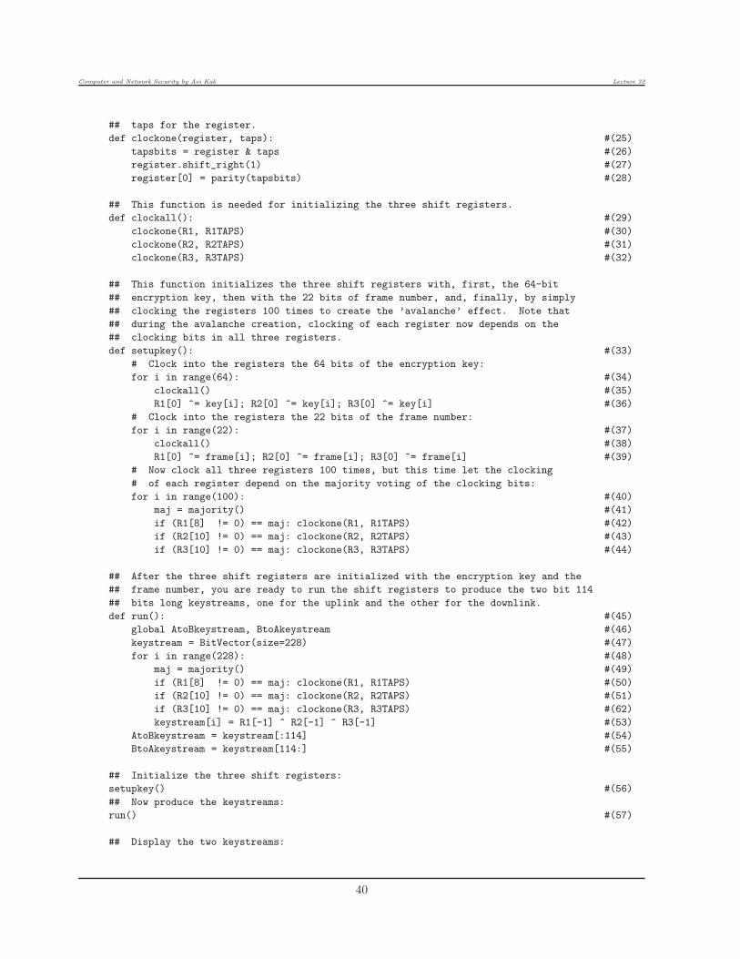
• The setupkey() in Lines (33) through (44) initializes the three
shift registers by, first, clocking in the 64 bits of the encryp-
tion key, then, by clocking in the 22 bits of the frame number,
and, finally, by simply clocking the registers 100 times for the
“avalanche” effect. Note the important difference between how
the registers are clocked in Lines (34) through (39) and in Lines
(40) through (44). In Lines (34) through (39), we clock all three
registers at each clock tick. However, in lines (40) through (44),
a register is clocked depending on how its clocking bit compares
with the clocking bits in other two registers.
37

Computer and Network Security by Avi Kak Lecture 32
• The function that actually produces the keystreams, run(), is de-
fined in Lines (45) through (55). I have combined the production
of the two keystreams into a single 228-iterations loop in Lines
(48) through (53). The first 114 bits generated in this manner are
for the uplink keystream and the next 114 bits for the downlink
keystream. This is reflected by the division made in lines (54)
and (55).
• The rest of the code is for checking the accuracy of the implemen-
tation against the test vector provided by Briceno et al. in their
C-based implementation. The variables goodAtoB and goodBtoA
store the correct values for the two keystreams for the encryption
key of Line (9) and the frame number of Line (12).
#!/usr/bin/env python
## A5_1.py
## Avi Kak ([email protected])
## April 21, 2015
## This is a Python implementation of the C code provided by Marc Briceno, Ian
## Goldberg, and David Wagner at the following website:
##
## http://www.scard.org/gsm/a51.html
##
## For accuracy, I have compared the output of this Python code against the test
## vector provided by them.
## The A5/1 algorithm is used in 2G GSM for over-the-air encryption of voice and SMS
## data. On the basis of the cryptanalysis of this cipher and the more recent
## rainbow table attacks, the A5/1 algorithm is now considered to provide virtually
## no security at all. Nonetheless, it forms an interesting case study that shows
## that when security algorithm are not opened up to public scrutiny (because some
## folks out there believe in "security through obscurity"), it is possible for such
## an algorithm to become deployed on a truly global basis before its flaws become
## evident.
38

Computer and Network Security by Avi Kak Lecture 32
## The A5/1 algorithm is a bit-level stream cipher based on three LFSR (Linear
## Feedback Shift Register). The basic operation you carry out in an LFSR at each
## clock tick consists of the following three steps: (1) You record the bits at the
## feedback taps in the register; (2) You shift the register by one bit position
## towards the MSB; and (3) You set the value of the LSB to an XOR of the feedback
## bits. When you are first initializing a register with the encryption key, you
## add a fourth step, which is to XOR the LSB with the key bit corresponding to that
## clock tick, etc.
from BitVector import *
# The three shift registers
R1,R2,R3 = BitVector(size=19),BitVector(size=22),BitVector(size=23) #(1)
# Feedback taps
R1TAPS,R2TAPS,R3TAPS = BitVector(size=19),BitVector(size=22),BitVector(size=23) #(2)
R1TAPS[13] = R1TAPS[16] = R1TAPS[17] = R1TAPS[18] = 1 #(3)
R2TAPS[20] = R2TAPS[21] = 1 #(4)
R3TAPS[7] = R3TAPS[20] = R3TAPS[21] = R3TAPS[22] = 1 #(5)
print "R1TAPS: ", R1TAPS #(6)
print "R2TAPS: ", R2TAPS #(7)
print "R3TAPS: ", R3TAPS #(8)
keybytes = [BitVector(hexstring=x).reverse() for x in [’12’, ’23’, ’45’, ’67’, \
’89’, ’ab’, ’cd’, ’ef’]] #(9)
key = reduce(lambda x,y: x+y, keybytes) #(10)
print "encryption key: ", key #(11)
frame = BitVector(intVal=0x134, size=22).reverse() #(12)
print "frame number: ", frame #(13)
## We will store the two output keystreams in these two BitVectors, each of size 114
## bits. One is for the uplink and the other for the downlink:
AtoBkeystream = BitVector(size = 114) #(14)
BtoAkeystream = BitVector(size = 114) #(15)
## This function used by the clockone() function. As each shift register is
## clocked, the feedback consists of the parity of all the tap bits:
def parity(x): #(16)
countbits = x.count_bits() #(17)
return countbits % 2 #(18)
## In order to decide whether or not a shift register should be clocked at a given
## clock tick, we need to examine the clocking bits in each register and see what the
## majority says:
def majority(): #(19)
sum = R1[8] + R2[10] + R3[10] #(20)
if sum >= 2: #(21)
return 1 #(22)
else: #(23)
return 0 #(24)
## This function clocks just one register that is supplied as the first arg to the
## function. The second argument must indicate the bit positions of the feedback
39
Computer and Network Security by Avi Kak Lecture 32
## taps for the register.
def clockone(register, taps): #(25)
tapsbits = register & taps #(26)
register.shift_right(1) #(27)
register[0] = parity(tapsbits) #(28)
## This function is needed for initializing the three shift registers.
def clockall(): #(29)
clockone(R1, R1TAPS) #(30)
clockone(R2, R2TAPS) #(31)
clockone(R3, R3TAPS) #(32)
## This function initializes the three shift registers with, first, the 64-bit
## encryption key, then with the 22 bits of frame number, and, finally, by simply
## clocking the registers 100 times to create the ’avalanche’ effect. Note that
## during the avalanche creation, clocking of each register now depends on the
## clocking bits in all three registers.
def setupkey(): #(33)
# Clock into the registers the 64 bits of the encryption key:
for i in range(64): #(34)
clockall() #(35)
R1[0] ^= key[i]; R2[0] ^= key[i]; R3[0] ^= key[i] #(36)
# Clock into the registers the 22 bits of the frame number:
for i in range(22): #(37)
clockall() #(38)
R1[0] ^= frame[i]; R2[0] ^= frame[i]; R3[0] ^= frame[i] #(39)
# Now clock all three registers 100 times, but this time let the clocking
# of each register depend on the majority voting of the clocking bits:
for i in range(100): #(40)
maj = majority() #(41)
if (R1[8] != 0) == maj: clockone(R1, R1TAPS) #(42)
if (R2[10] != 0) == maj: clockone(R2, R2TAPS) #(43)
if (R3[10] != 0) == maj: clockone(R3, R3TAPS) #(44)
## After the three shift registers are initialized with the encryption key and the
## frame number, you are ready to run the shift registers to produce the two bit 114
## bits long keystreams, one for the uplink and the other for the downlink.
def run(): #(45)
global AtoBkeystream, BtoAkeystream #(46)
keystream = BitVector(size=228) #(47)
for i in range(228): #(48)
maj = majority() #(49)
if (R1[8] != 0) == maj: clockone(R1, R1TAPS) #(50)
if (R2[10] != 0) == maj: clockone(R2, R2TAPS) #(51)
if (R3[10] != 0) == maj: clockone(R3, R3TAPS) #(62)
keystream[i] = R1[-1] ^ R2[-1] ^ R3[-1] #(53)
AtoBkeystream = keystream[:114] #(54)
BtoAkeystream = keystream[114:] #(55)
## Initialize the three shift registers:
setupkey() #(56)
## Now produce the keystreams:
run() #(57)
## Display the two keystreams:
40

Computer and Network Security by Avi Kak Lecture 32
print "\nAtoBkeystream: ", AtoBkeystream #(58)
print "\nBtoAkeystream: ", BtoAkeystream #(59)
## Here are the correct values for the two keystreams:
goodAtoB = [BitVector(hexstring = x) for x in [’53’,’4e’,’aa’,’58’,’2f’,’e8’,’15’,’1a’,\
’b6’,’e1’,’85’,’5a’,’72’,’8c’,’00’] ] #(60)
goodBtoA = [BitVector(hexstring = x) for x in [’24’,’fd’,’35’,’a3’,’5d’,’5f’,’b6’,’52’,\
’6d’,’32’,’f9’,’06’,’df’,’1a’,’c0’] ] #(61)
goodAtoB = reduce(lambda x,y: x+y, goodAtoB) #(62)
goodBtoA = reduce(lambda x,y: x+y, goodBtoA) #(63)
print "\nGood: AtoBkeystream: ", goodAtoB[:114] #(64)
print "\nGood: BtoAkeystream: ", goodBtoA[:114] #(65)
if (AtoBkeystream == goodAtoB[:114]) and (AtoBkeystream == goodAtoB[:114]): #(66)
print "\nSelf-check succeeded: Everything looks good" #(67)
• When you run this code, you should see the following output
R1TAPS: 0000000000000100111
R2TAPS: 0000000000000000000011
R3TAPS: 00000001000000000000111
encryption key: 0100100011000100101000101110011010010001110101011011001111110111
frame number: 0010110010000000000000
AtoBkeystream: 010100110100111010101010010110000010111111101000000101010001
101010110110111000011000010101011010011100101000110000
BtoAkeystream: 001001001111110100110101101000110101110101011111101101100101
001001101101001100101111100100000110110111110001101011
Good AtoBkeystream: 010100110100111010101010010110000010111111101000000101010001
101010110110111000011000010101011010011100101000110000
Good BtoAkeystream: 001001001111110100110101101000110101110101011111101101100101
001001101101001100101111100100000110110111110001101011
Self-check succeeded: Everything looks good
• You are probably wondering as to why I did not show the keystreams
in hex. In general, you can display a BitVector object in hex by
41
Computer and Network Security by Avi Kak Lecture 32
calling its instance method get hex from bitvector() — provided
the number of bits is a multiple of 4. Our keystreams are 114 bits
long, which is not a multiple of 4. I could have augmented the
keystreams by appending a couple of zeros at the end, but then
you are taking liberties with the correctness of the output.
42
Computer and Network Security by Avi Kak Lecture 32
32.5: SIDE-CHANNEL ATTACKS ONSPECIALIZED MOBILE DEVICES
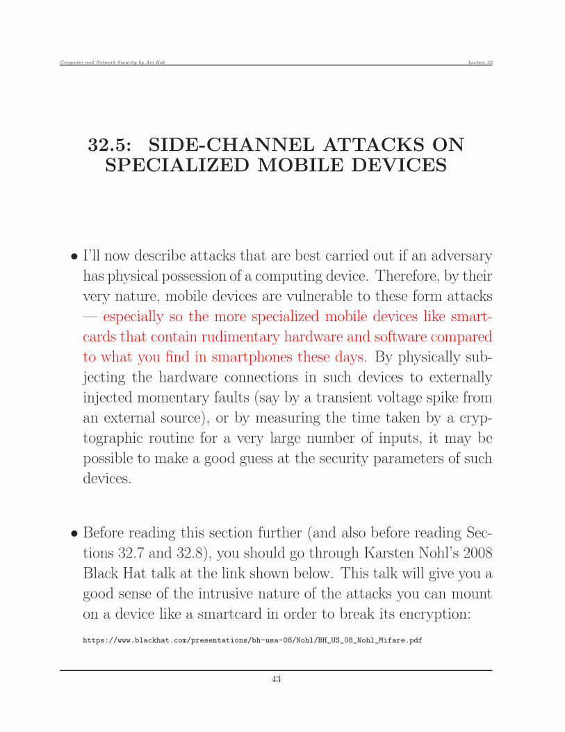
• I’ll now describe attacks that are best carried out if an adversary
has physical possession of a computing device. Therefore, by their
very nature, mobile devices are vulnerable to these form attacks
— especially so the more specialized mobile devices like smart-
cards that contain rudimentary hardware and software compared
to what you find in smartphones these days. By physically sub-
jecting the hardware connections in such devices to externally
injected momentary faults (say by a transient voltage spike from
an external source), or by measuring the time taken by a cryp-
tographic routine for a very large number of inputs, it may be
possible to make a good guess at the security parameters of such
devices.
• Before reading this section further (and also before reading Sec-
tions 32.7 and 32.8), you should go through Karsten Nohl’s 2008
Black Hat talk at the link shown below. This talk will give you a
good sense of the intrusive nature of the attacks you can mount
on a device like a smartcard in order to break its encryption:
https://www.blackhat.com/presentations/bh-usa-08/Nohl/BH_US_08_Nohl_Mifare.pdf
43

Computer and Network Security by Avi Kak Lecture 32
• In general, a side-channel attack means that an adversary is try-
ing to break a cipher using information that is NOT intrinsic
to the mathematical details of the encryption/decryption algo-
rithms, but that may be inferred from various “external” mea-
surements such as the power consumed by the hardware executing
the algorithms for different possible inputs, the time taken by the
hardware for the same, how the hardware responds to externally
injected faults, etc.
• Various forms of side-channel attacks are:
Fault Injection Attack: These are based on deliberately get-
ting the hardware on which a specific part of encryption/decryption
algorithm is running to return a wrong answer. As shown in
the next section, a wrong answer may give sufficient clues to
figure out the parameters of the cryptographic algorithm being
used.
Timing Attack: These attacks try to infer a cryptographic key
from the time it takes for the processor to execute an algorithm
and the dependence of this time on different inputs.
Power Analysis Attack: Here the goal is to analyze the power
trace of an executing cryptographic algorithm in order to fig-
ure out whether a particular instruction was executed at a
specific time. It has been shown that such traces can reveal
44
Computer and Network Security by Avi Kak Lecture 32
the cryptographic keys used.
EM Analysis Attack: Assuming that the hardware implement-
ing a cryptographic routine is not adequately shielded against
leaking electromagnetic radiation (at the clock frequency of
the processor), if you can construct a trace of this radiation,
you may be able to infer whether or not a particular instruc-
tion was executed at a given time — just as in a power analysis
attack. From such information, you may be able to draw in-
ferences about the bits in a encryption key.
• In the sections that follow, I will consider two of these attacks in
greater detail: the fault-injection attack and the timing attack. In
order to explain the principles involved, for both these attacks, I
will assume that a mobile device is charged with digitally signing
the outgoing messages with the RSA algorithm. The goal of
the attacks will be make a guess at the private exponent used for
constructing a digital signature. Note that these days if an attack
can reliably guess even a single bit of a secret, it is considered
to be a successful attack.
45
Computer and Network Security by Avi Kak Lecture 32
32.6: FAULT INJECTION ATTACKS
• The goal of this section is to show that if you can get the processor
of a mobile device to yield a faulty value for a portion of the
calculations, you may be able to get the device to part with its
secret, which could be the encryption key you are looking for.
• I will assume that the processor of the mobile device has an em-
bedded private key for digitally signing messages with the RSA
algorithm.
• The reader will recall from Lecture 12 that given a modulus n
and a public and private key pair (e, d), we can sign a message
M by calculating its digital signature S = Md mod n. [In practice,
you are likely to calculate the signature of just the hash of the message M . That detail, however, does not
change the overall explanation presented in this section.]
• As explained in Section 12.5 of Lecture 12, calculation of the
signature S = Md (mod n) can be speeded up considerably by
using the Chinese Remainder Theorem (CRT). Since the owner
of the private key d will also know the prime factors p and q of
46

Computer and Network Security by Avi Kak Lecture 32
the modulus n, with CRT you first calculate [In the explanation in Section
12.5 of Lecture 12, our focus was on encryption/decryption with RSA. Therefore, the private exponent d was
applied to the ciphertext integer C. Here we are talking about digital signatures, which calls for applying the
private exponent to the message itself (or to a hash of the message).]
Vp = Md mod p
Vq = Md mod q
In order to construct the signature S from Vp and Vq, we must
calculate the coefficients:
Xp = q × (q−1 mod p)
Xq = p× (p−1 mod q)
The CRT theorem of Section 11.7 of Lecture 11 then tells us that
the signature S is related to the intermediate results Vp and Vq
by
S =(
Vp ×Xp + Vq ×Xq
)
mod n
=
(
q × (q−1 mod p)× Vp + p× (p−1 mod q)× Vq
)
mod n (1)
• Let’s now assume that we have somehow introduced a fault in the
calculation of Vp by, say, subjecting the hardware to a momentary
voltage surge. Since the voltage surge is limited in duration, we
assume that while Vp is now calculated erroneously as Vp, the
value of Vq remains unchanged. Let’s use S to represent the
signature calculated using the erroneous Vp. We can write:
47

Computer and Network Security by Avi Kak Lecture 32
S =
(
q × (q−1 mod p)× Vp + p× (p−1 mod q)× Vq
)
mod n
• Subtracting the faulty signature S from its true value S, we have
S − S =
(
q × (q−1 mod p)[Vp − Vp]
)
mod n (2)
• The above result implies that
q = gcd(S − S, n) (3)
As you can see, the attacker can immediately figure out the
prime factor q of the modulus by calculating the GCD of S − S
and n. [See Lecture 5 for how to best calculate the GCD of two numbers.] Subsequently,
a simple division would yield to the attacker the other prime
factor p. In this manner, the attacker would be able to figure
out the prime factors of the RSA modulus without ever having
to factorize it. After acquiring the prime factors p and q, it
becomes a trivial matter for the attacker to find out what the
private key d is since the attacker knows the public key e.
• The ploy described above requires that the attacker calculate both
the true signature S and the faulty signature S for a messageM .
As it turns out, the attacker can carry out the same exploit with
just the faulty signature S along with the message M .
48

Computer and Network Security by Avi Kak Lecture 32
• To see why the same exploit works with M and S, note first thatif we are given the correct signature S, we can recover M byM = Se mod n. Also note that since Se mod n = M , we canwrite:
Se = k1 × n + M
= k1 × p× q + M
for some value of the integer constant k1. The second relationshipshown above leads to:
Se mod p = M (4)
Se mod q = M (5)
• Also note that, using Equation (1), we can write for the correctsignature:
S =
(
q × (q−1 mod p)× Vp + p× (p−1 mod q)× Vq
)
mod n
= q × (q−1 mod p)× Vp + p× (p−1 mod q)× Vq + k2 × p× q
for some value of the constant k2. We can therefore write:
Se =
(
q × (q−1 mod p)× Vp + p× (p−1 mod q)× Vq + k2 × p× q
)e
and that implies
49

Computer and Network Security by Avi Kak Lecture 32
Se mod p =
(
q × (q−1 mod p)× Vp + p× (p−1 mod q)× Vq + k2 × p× q
)e
mod p
=
((
q × (q−1 mod p)× Vp + p× (p−1 mod q)× Vq + k2 × p× q
)
mod p
)e
mod p
=
(
q × (q−1 mod p)× Vp
)e
mod p (6)
We can derive a similar result for Se mod q. Writing the two
results together, we have
Se mod p =
(
q × (q−1 mod p)× Vp
)e
mod p = M (7)
Se mod q =
(
p× (p−1 mod q)× Vq
)e
mod q = M (8)
where we have also placed the result derived earlier in Equations
(4) and (5).
• Let’s now try to see what happens if carry out similar operations
on the faulty signature S. However, before we raise S to the
power e, let’s rewrite S as
S =
(
q × (q−1 mod p)× Vp + p× (p−1 mod q)× Vq
)
mod n
= q × (q−1 mod p)× Vp + p× (p−1 mod q)× Vq + k3 × p× q
for some value of the integer k3. We may now write for Se:
Se =
(
q × (q−1 mod p)× Vp + p× (p−1 mod q)× Vq + k3 × p× q
)e
50

Computer and Network Security by Avi Kak Lecture 32
This allows us to write:
Se mod p =
(
q × (q−1 mod p)× Vp + p× (p−1 mod q)× Vq + k3 × p× q
)e
mod p
=
((
q × (q−1 mod p)× Vp + p× (p−1 mod q)× Vq + k3 × p× q
)
mod p
)e
mod p
=
(
q × (q−1 mod p)× Vp
)e
mod p (9)
• In a similar manner, one can show
Se mod q =
(
p× (p−1 mod q)× Vq
)e
mod q (10)
• Comparing the results in Equations (6) and (7) with those in
Equations (4) and (5), we claim
Se mod p 6= M (11)
Se mod q = M (12)
• Equation (9) implies that we can write
Se = M + k4 × q (13)
for some value of the constant k4. This relationship may be
expressed as
51

Computer and Network Security by Avi Kak Lecture 32
Se − M = k4 × q (14)
• Since n = p× q, what we have is that Se −M and the modulus
n share common factor, q. Since n possesses only two factors, p
and q, we can therefore write
gcd(Se − M,n) = q (15)
52

Computer and Network Security by Avi Kak Lecture 32
32.6.1: Demonstration of Fault Injection with a
Python Script
• The goal of this demonstration is to illustrate that when you
miscalculate (deliberately) either Vp or Vq in the CRT step of the
modular exponentiation required by the RSA algorithm, you can
easily figure out the private key d.
• In the Python script that follows, lines (1) through (18) show two
functions, gcd() and MI() that you saw previously in Lecture 5.
The gcd() is the Euclid’s algorithm for calculating the greatest
common divisor of two integers. And the function MI() returns
the multiplicative inverse of the first-argument integer in the ring
corresponding to the second-argument integer.
• Subsequently, lines (19) through (29) first declare the two prime
factors for the RSA modulus and then compute the values to
use for the public exponent e and the private exponent d. As
the reader will recall from Section 12.2.2 of Lecture 12, e must
be relatively prime to both p − 1 and q − 1, which are the two
factors of the totient of n. The conditional evaluation in line (25)
guarantees that. After setting e, the statement in line (28) sets
the private exponent d.
53

Computer and Network Security by Avi Kak Lecture 32
• The code in lines (30) through (37) first sets the message integer
M and then calculates the intermediate results Vp and Vq, as de-
fined in the previous section. Note that we use Fermat’s Little
Theorem (see Section 11.2 of Lecture 11) to speed up the calcula-
tion of Vp and Vq. [Given the small sizes of the numbers involved, there is obviously no particular
reason to use FLT here. Nonetheless, should be reader decide to play with this demonstration using large num-
bers, using FLT would certainly make for a faster response time from the demonstration code.] In line
(36), we use the CRT theorem to combine the values for Vp and
Vq into the RSA based digital signature of the message integer
M .
• Finally, the code in lines (39) through (47) is the demonstration
of fault injection and how it can be used to find the prime factor
q of the RSA modulus n. We simulate fault injection by adding
a small random number to the value of Vp in line (42). Subse-
quently, we use Equation (10) of the previous section to estimate
the value for q in line (44).
#!/usr/bin/env python
## FaultInjectionDemo.py
## Avi Kak (March 30, 2015)
## This script demonstrates the fault injection exploit on the CRT step of the
## of the RSA algorithm.
## GCD calculator (From Lecture 5)
def gcd(a,b): #(1)
while b: #(2)
a,b = b, a%b #(3)
return a #(4)
## The code shown below uses ordinary integer arithmetic implementation of
## the Extended Euclid’s Algorithm to find the MI of the first-arg integer
## vis-a-vis the second-arg integer. (This code segment is from Lecture 5)
54

Computer and Network Security by Avi Kak Lecture 32
def MI(num, mod): #(5)
’’’
The function returns the multiplicative inverse (MI) of num modulo mod
’’’
NUM = num; MOD = mod #(6)
x, x_old = 0L, 1L #(7)
y, y_old = 1L, 0L #(8)
while mod: #(9)
q = num // mod #(10)
num, mod = mod, num % mod #(11)
x, x_old = x_old - q * x, x #(12)
y, y_old = y_old - q * y, y #(13)
if num != 1: #(14)
raise ValueError("NO MI. However, the GCD of %d and %d is %u" \
% (NUM, MOD, num)) #(15)
else: #(16)
MI = (x_old + MOD) % MOD #(17)
return MI #(18)
# Set RSA params:
p = 211 #(19)
q = 223 #(20)
n = p * q #(21)
print "RSA parameters:"
print "p = %d q = %d modulus = %d" % (p, q, n) #(22)
totient_n = (p-1) * (q-1) #(23)
# Find a candidate for public exponent:
for e in range(3,n): #(24)
if (gcd(e,p-1) == 1) and (gcd(e,q-1) == 1): #(25)
break #(26)
print "public exponent e = ", e #(27)
# Now set the private exponent:
d = MI(e, totient_n) #(28)
print "private exponent d = ", d #(29)
message = 6789 #(30)
print "\nmessage = ", message #(31)
# Implement the Chinese Remainder Theorem to calculate
# message to the power of d mod n:
dp = d % (p - 1) #(32)
dq = d % (q - 1) #(33)
V_p = ((message % p) ** dp) % p #(34)
V_q = ((message % q) ** dq) % q #(35)
signature = (q * MI(q, p) * V_p + p * MI(p, q) * V_q) % n #(36)
print "\nsignature = ", signature #(37)
import random #(38)
print "\nESTIMATION OF q THROUGH INJECTED FAULTS:"
for i in range(10): #(39)
55

Computer and Network Security by Avi Kak Lecture 32
error = random.randrange(1,10) #(40)
V_hat_p = V_p + error #(42)
print "\nV_p = %d V_hat_p = %d error = %d" % (V_p, V_hat_p, error) #(41)
signature_hat = (q * MI(q, p) * V_hat_p + p * MI(p, q) * V_q) % n #(43)
q_estimate = gcd( (signature_hat ** e - message) % n, n) #(44)
print "possible value for q = ", q_estimate #(45)
if q_estimate == q: #(46)
print "Attack successful!!!" #(47)
• Shown below is the output of the script. As the reader can see,
for all values of the random error added to the value of Vp, we are
able to correctly estimate the prime factor q of the RSA modulus.
RSA parameters:
p = 211 q = 223 modulus = 47053
public exponent e = 11
private exponent d = 21191
message = 6789
signature = 42038
ESTIMATION OF q THROUGH INJECTED FAULTS:
V_p = 49 V_hat_p = 56 error = 7
possible value for q = 223
Attack successful!!!
V_p = 49 V_hat_p = 55 error = 6
possible value for q = 223
Attack successful!!!
V_p = 49 V_hat_p = 53 error = 4
possible value for q = 223
Attack successful!!!
V_p = 49 V_hat_p = 52 error = 3
possible value for q = 223
Attack successful!!!
56

Computer and Network Security by Avi Kak Lecture 32
V_p = 49 V_hat_p = 54 error = 5
possible value for q = 223
Attack successful!!!
V_p = 49 V_hat_p = 52 error = 3
possible value for q = 223
Attack successful!!!
V_p = 49 V_hat_p = 53 error = 4
possible value for q = 223
Attack successful!!!
V_p = 49 V_hat_p = 56 error = 7
possible value for q = 223
Attack successful!!!
V_p = 49 V_hat_p = 58 error = 9
possible value for q = 223
Attack successful!!!
V_p = 49 V_hat_p = 58 error = 9
possible value for q = 223
Attack successful!!!
• Fault injection attacks were first discovered by Dan Boneh, Richard
DeMillo, and Richard Lipton in 1997 and are described in their
2001 Journal of Cryptology publication “On the Importance of
Eliminating Errors in Cryptographic Computations.” The logic
used in the Python script shown in this section is based on a re-
finement of the original attack by A. K. Lenstra. This refinement
is also mentioned in the publication by Boneh et al.
57

Computer and Network Security by Avi Kak Lecture 32
32.7: TIMING ATTACKS
• Timings attacks are based on the premise that if you can monitor
how long it takes to execute a certain segment of a cryptographic
routine, you may be able to make a good guess for the secret
parameters of the algorithm.
• To elaborate, let’s consider the following algorithm for modularexponentiation that you saw earlier in Section 12.5.1 of Lecture12: [The Fault Injection discussion in Section 32.6 of the current lecture focused on the CRT step of
the overall implementation of a modular exponentiation algorithm. As you will recall from Section 12.5.1 of
Lecture 12, after you have carried out the simplification of modular exponentiation with CRT, you still need
to calculate a quantity like AB
mod n.]
result = 1
while B > 0:
if B & 1: #(1)
result = ( result * A ) % n #(2)
B = B >> 1
A = ( A * A ) % n
return result
As explained in Section 12.5.1 of Lecture 12, this algorithm carries
out a bitwise scan of the exponent B from its least significant bit
to its most significant bit. It calculates the square of the base A
58

Computer and Network Security by Avi Kak Lecture 32
at each step of the scan. This squared value is multiplied with the
intermediate value for the result only if the bit of the exponent
is set at the current step.
• Now imagine that you have somehow acquired the means to mon-
itor how long it takes to execute the code in lines (1) and (2)
shown above. Assuming that your time measurements are rea-
sonably accurate, these time measurements would directly yield
the exponent B. And even if your time measurements are not so
reliable, perhaps you can carry out the exponentiation operation
repeatedly and then average out the noise. This is exactly the
basis for the demonstration in the Python script shown next.
• Obviously, your first reaction to the claim made above would
be: How would you get inside the hardware of a mobile device
to monitor the execution time of the code segments in order to
infer the secret through the time taken by those portions of the
code? In practically all situations, the most an attacker would
be able to do would be to feed different messages into a mobile
device and measure the total time taken by an algorithm for each
of those messages. Subsequently, if at all possible, the attacker
would need to infer the secret from those times.
• The goal of the subsection that follows is to show that it is possi-
ble to determine an encryption key from the overall time taken
by algorithm for each of a large collection of randomly constructed
59

Computer and Network Security by Avi Kak Lecture 32
messages.
• The goal of the current section, however, is simply to focus on
showing how one can measure the execution time associated with
a code fragment and the averaging that is needed to mitigate the
effects of noise associated with such measurements.
• Let’s now address the question of how one might measure the time
associated with the execution of an entire algorithm, or with just a
fragment of the code, and why such measurements are inherently
noisy. You might try to measure the execution time by taking the
difference of the wall clock time just before the entry into the code
segment and just after exiting from that code segment. Such an
estimate is bound to be merely an approximation to the actual
time spent in the processor by that segment of code. You see, at
any given instant of time, there could be tens, if not hundreds, of
processes and threads running “concurrently” in your computer.
Assuming for the sake of argument that you have a single-core
processor, what that means is that all the processes and threads
are time-sliced with regard to their access to the CPU. That is, a
process or a thread currently being executed in the CPU is rolled
out and its state saved in the memory when the quantum of time
for which it is allowed to be executed expires. Subsequently, one
of the waiting processes or threads is rolled into the CPU, and
so on. [All modern operating systems maintain several queues for the concurrent execution of multiple
processes and threads. There is, for example, a queue of processes that are waiting for their turn at the CPU.
Should a process that is currently being executed by the CPU need access to a particular I/O device, it is
60

Computer and Network Security by Avi Kak Lecture 32
taken off the CPU and placed in a queue for that I/O device. After it is done with I/O, it goes back into
the queue of the processes waiting for their turn at the CPU. Unless a process is taken off the CPU for I/O
reasons, or because it has been interrupted, etc., more ordinarily a process is taken off the CPU because its
allotted time-slice in the CPU has expired. In Unix/Linux systems, there is a special process of PID 0 that
acts as a processor scheduler. The scheduler’s job is to figure out which of the waiting processes gets a turn at
the CPU.]
• To demonstrate how noisy the measurement of running time can
be, shown below are 10 trials of the same algorithm that consists
of 16 steps. The execution time of each step was measured as
the difference between the wall-clock time before and after the
execution of the code segment corresponding to that step. That
several of the entries are ‘0.0’ is not surprising because 12 of the
16 steps are essentially do-nothing step. However, the remain-
ing four do require a large multiplication. The four steps that
involve a large multiplication are at the first, eighth, tenth, and
the sixteenth steps.
#1: [5.96e-06, 0.0, 0.0, 0.0, 9.53e-07, 0.0, 0.0, 0.0, 9.53e-07, 0.0, 0.0, 9.53e-07, 0.0, 9.53e-07, 0.0, 0.0]
#2: [5.96e-06, 9.53e-07, 9.53e-07, 0.0, 0.0, 9.53e-07, 0.0, 0.0, 9.53e-07, 0.0, 0.0, 9.53e-07, 0.0, 0.0, 0.0, 0.0]
#3: [5.96e-06, 9.53e-07, 9.53e-07, 0.0, 0.0, 9.53e-07, 0.0, 0.0, 0.0, 0.0, 9.53e-07, 0.0, 0.0, 0.0, 0.0, 1.19e-06]
#4: [5.96e-06, 9.53e-07, 0.0, 0.0, 0.0, 0.0, 1.19e-06, 0.0, 0.0, 0.0, 0.0, 0.0, 0.0, 0.0, 1.19e-06, 0.0]
#5: [5.96e-06, 9.53e-07, 0.0, 0.0, 0.0, 0.0, 0.0, 0.0, 9.53e-07, 1.19e-06, 0.0, 0.0, 0.0, 0.0, 0.0, 0.0]
#6: [5.96e-06, 0.0, 0.0, 0.0, 0.0, 0.0, 1.19e-06, 0.0, 0.0, 0.0, 9.53e-07, 0.0, 9.53e-07, 0.0, 0.0, 0.0]
#7: [5.96e-06, 9.53e-07, 9.53e-07, 0.0, 0.0, 0.0, 0.0, 0.0, 9.53e-07, 0.0, 0.0, 9.53e-07, 0.0, 9.53e-07, 0.0, 0.0]
#8: [5.96e-06, 0.0, 0.0, 0.0, 0.0, 0.0, 9.53e-07, 0.0, 0.0, 0.0, 0.0, 0.0, 0.0, 0.0, 0.0, 0.0]
#9: [8.10e-06, 0.0, 0.0, 0.0, 9.53e-07, 0.0, 0.0, 0.0, 9.53e-07, 0.0, 0.0, 0.0, 1.19e-06, 0.0, 0.0, 9.53e-07]
#10: [6.19e-06, 0.0, 0.0, 0.0, 0.0, 0.0, 9.53e-07, 0.0, 0.0, 0.0, 0.0, 0.0, 0.0, 0.0, 0.0, 0.0]
61

Computer and Network Security by Avi Kak Lecture 32
• Our goal in this section is to illustrate how to recover the value of
the exponent B in the computation of AB mod n from the noisy
execution times of one key step in the modular exponentiation
algorithm shown in the previous section.
• In the script that follows, lines (1) through (12) define the same
modular exponentiation algorithm you saw earlier — except for
the time measurement statements that are interspersed. The time
measurement statements are in lines (2), (5), (8), and (9). We
want to measure the time it takes to compute the multiplication
step in line (7) recognizing that this multiplication takes place
subject to the condition in line (6). The number of iterations in
the while loop that starts in line (4) is equal to the number of
bits in the binary representation of the exponent B.
• Subsequently, in order to deal with the noise in the measure-
ment of execution time as demonstrated in the previous sec-
tion, we define the function repeated time measurements()
in lines (13) through (20). All that this function does is to
call the modular exponentiation function repeatedly. It is the
third argument to repeated time measurements() that de-
termines how many times the modular exponentiation function
will be called. The time measurements in each call to modular
exponentiation are stored in a list of lists bound to the variable
list of time traces.
• In lines (21) through (24), we then set the values for the base A,
62

Computer and Network Security by Avi Kak Lecture 32
the exponent B, the modulus n, and the number of repetitions
for calling the modular exponentiation function. In line (25), we
then call repeated time measurements() with these values.
• The rest of the code, in lines (26) through (38), is for first aver-
aging the noisy time measurements for each of the steps, finding
a threshold as the half-way point between the minimum and the
maximum of the time measurements, thresholding the time mea-
surements, and constructing a bit string from the 0’s and 1’s thus
obtained.
#!/usr/bin/env python
## EstimatingExponentFromExecutionTime.py
## Avi Kak ([email protected])
## March 31, 2015
## This script demonstrates the basic idea of how it is possible to infer
## the bit field of an exponent by measuring the time it takes to carry
## out the one of the key steps in the modular exponentiation algorithm.
import time
## This is our basic script for modular exponentiation. See Section 12.5.1 of
## Lecture 12:
def modular_exponentiate(A, B, modulus): #(1)
time_trace = [] #(2)
result = 1 #(3)
while B > 0: #(4)
start = time.time() #(5)
if B & 1: #(6)
result = ( result * A ) % modulus #(7)
elapsed = time.time() - start #(8)
time_trace.append(elapsed) #(9)
B = B >> 1 #(10)
A = ( A * A ) % modulus #(11)
return result, time_trace #(12)
## Since a single experiment does not yield reliable measurements of the time
## taken by a computational step, this function helps us carry out repeated
## experiments:
63

Computer and Network Security by Avi Kak Lecture 32
def repeated_time_measurements(A, B, modulus, how_many_times): #(13)
list_of_time_traces = [] #(14)
results = [] #(15)
for i in range(how_many_times): #(16)
result, timetrace = modular_exponentiate(A, B, modulus) #(17)
list_of_time_traces.append(timetrace) #(18)
results.append(result) #(19)
# Also return ‘results’ for debugging, etc.
return list_of_time_traces, results #(20)
A = 123456789012345678901234567890123456789012345678901234567890 #(21)
B = 0b1111110101001001
modulus = 987654321 #(23)
num_iterations = 1000 #(24)
list_of_time_traces, results = repeated_time_measurements(A, B, modulus, num_iterations)#(25)
sums = [sum(e) for e in zip(*list_of_time_traces)] #(26)
averages = [x/num_iterations for x in sums] #(27)
averages = list(reversed(averages)) #(28)
print "\ntimings: ", averages #(29)
minval, maxval = min(averages), max(averages) #(30)
threshold = (maxval - minval) / 2 #(31)
bitstring = ’’ #(32)
for item in averages: #(33)
if item > threshold: #(34)
bitstring += ’1’ #(35)
else: #(36)
bitstring += ’0’ #(37)
print "\nbitstring for B constructed from timings: ", bitstring #(38)
• If you run the Python script as shown above, it outputs the bit
string:
1111110101001001
which is the same as the bit pattern for the exponent in line
(22). You can run the same experiment with other choices for
the exponent B in line (22). For example, if I change that line
to B = 0b1100110101110101, the answer returned by the script is
1100110101110101, and so on.
64

Computer and Network Security by Avi Kak Lecture 32
• This establishes that, despite the inherently noisy nature of
time measurements, you can figure out the value of the expo-
nent in a modular exponentiation required for a cryptographic
calculation just by measuring how long it takes to execute one of
the key steps of the algorithm.
• That it may be possible to mount the timing attack on a cryp-
tographic routine was first conjectured by Paul Kocher in 1996
in a paper entitled “Timing Attacks on Implementations of Diffie-
Hellman, RSA, DSS, and Other Systems,” that appeared in CRYPTO’96,
Lecture Notes in Computer Science, Vol. 1355.
• Keeping these considerations in mind, the next subsection demon-
strates the basic elements of a Timing Attack with the help of a
Python script.
65

Computer and Network Security by Avi Kak Lecture 32
32.7.1: A Python Script That Demonstrates How To
Use Code Execution Time for Mounting a Timing
Attack
• Let’s now talk about how to actually mount a timing attack using
the times required for fully computing the RSA signatures for a
collection of randomly constructed messages. In other words, we
will no longer assume that we can measure the times taken by
the individual steps of the modular exponentiation algorithm.
• As matters stand today, for a serious attempt at mounting a
timing attack, we will need to implement it in a way that is
described in the paper “A Practical Implementation of the Tim-
ing Attack” by Jean-Francois Dhem, Francois Koeune, Philippe-
Alexandre Leroux, Patrick Mestre, Jean-Jacques Quisquater, and
Jean-Louis Willems that appeared in the Proceedings of the In-
ternational Conference on Smart Cards and Applications, 1998,
pp. 167-182. [This is a probabilistic approach that entails: (1) scanning the bit positions in an
encryption key from right to left; (2) forming two hypotheses at each bit position, one for the bit being 0 and
the other for the bit being 1; (3) Finding probabilistic support for each hypothesis taking into account the bits
discovered so far, and the difference between the sizes of the message populations under the two hypotheses
(membership in the populations takes into account the fact that the hypothesis that calls for the bit to be
1 would entail a slightly longer computation).] Using this approach, the authors
were able to break a 512-bit key in a few minutes using 300,000
timing measurements.
66

Computer and Network Security by Avi Kak Lecture 32
• My goal in this section is not to replicate the work described in the
publication cited above. On the other hand, all I want to show is
that there exist correlations between the time measurements for
modular exponentiation for a collection of randomly constructed
messages and the times measured for the same exponentiations
under the hypothesis that a particular bit in the exponent is 1
or 0. Further, that these correlations can be exploited to makes
guesses for the individual bits of the exponent.
• In order to frame the problem that the Python script in this sec-
tion tries to solve with a toy implementation, let’s go back to the
case of a device that uses the RSA algorithm to digitally sign the
outgoing messages. As stated earlier, given a messageM and the
private exponent d, this device must compute Md mod n where
n is the RSA modulus. Earlier, in Section 32.6.1, we saw how the
CRT step that is used to simplify the modular exponentiation
can be subject to fault injection for discovering the value of the
private key.
• We will now assume that we are directly computing modular
exponentiationMd mod n required for digitally signing a message
M with a private exponent d. Our goal is to discover d just
from the time it takes to calculate the signatures for an arbitrary
collection of messages. As will always be the case, we will assume
that d is odd and, therefore, its least significant bit is always 1.
Our goal is to discover the rest of the bits.
67

Computer and Network Security by Avi Kak Lecture 32
• The overall logic of the script is to estimate the bits of the private
exponent d, one bit at a time, starting from its least significant
bit (which, as already mentioned, is 1). The estimation is based
on finding correlations between the times taken to calculate the
signatures under two conditions: when the bit to be estimated can
be assumed to be 0 and when it can be assumed to be 1. Under
each hypothesis, the correlation is with the time measurements
for the actual signature computations. We declare a value for the
next bit on the basis of which correlation is larger.
• The workhorse in the script that follows is the method find next
bit of private key(). Its two main blocks are in lines (F9)
through (F25) and in lines (F33) through (F46). In the first
block, in lines (F9) through (F25), this function calculates the
correlation for the case when we assume 0 for the next bit po-
sition in the private exponent d. In the second block, in lines
(F33) through (F46), we calculate a similar correlation for the
case when we assume the next bit to be 1. The two correlation
values are compared in line (F47).
• You have to use a very large number of message integers for the
attack to work to any extent at all. As you will notice from the
constructor call in lines (A1) through (A6), my own experiments
with this script typically involve 100,000 message integers.
• You might think that in the multiple runs of the overall attack
in lines (A9) through (A25), we could speed up the overall time
68

Computer and Network Security by Avi Kak Lecture 32
taken by the script by placing the call that generates the very
large number of messages in line (A11) outside the loop. Note
that the time taken to generate 100,000 messages is a very small
fraction of the time taken by the modular exponentiation of those
messages through the code in lines (X1) through (X11).
• The dictionary bound to the instance variable correlations
cache in line (J15) is used in find next bit of private key()
in lines (F8) and (F30). This dictionary helps avoid duplicating
the correlation calculations for the same value of the private ex-
ponent.
#!/usr/bin/env python
## TimingAttack.py
## Avi Kak ([email protected])
## April 13, 2015
## This script demonstrates the basic idea of how the Timing Attack can be
## used to infer the bits of the private exponent used in calculating RSA
## based digital signatures.
##
## CAVEATS: This simple implementation is based on one possible
## interpretation of the original paper on timing attacks by Paul
## Kocher. Note that this implementation has only been tried on
## 8-bit moduli.
##
## I am quite certain that this extremely simpleminded implementation
## will NOT to work on RSA moduli of the size that are actually used
## in working algorithms.
##
## For a more credible timing attack, you would need to include
## in this implementation the probabilstic logic described in the
## paper "A Practical Implementation of the Timing Attack’’ by
## Dhem, Koeune, Leroux, Mestre, Quisquater, and Willems.
import time
import random
import math
69

Computer and Network Security by Avi Kak Lecture 32
class TimingAttack( object ): #(I1)
def __init__( self, **kwargs ): #(J2)
if kwargs.has_key(’num_messages’): num_messages = kwargs.pop(’num_messages’) #(J3)
if kwargs.has_key(’num_trials’): num_trials = kwargs.pop(’num_trials’) #(J3)
if kwargs.has_key(’private_exponent’): private_exponent = kwargs.pop(’private_exponent’)
#(J4)
if kwargs.has_key(’modulus_width’): modulus_width = kwargs.pop(’modulus_width’) #(J5)
self.num_messages = num_messages #(J6)
self.num_trials = num_trials #(J7)
self.modulus_width = modulus_width #(J8)
self.d = private_exponent #(J9)
self.d_reversed = ’{:b}’.format(private_exponent)[::-1] #(J10)
self.modulus = None #(J11)
self.list_of_messages = [] #(J12)
self.times_taken_for_messages = [] #(J13)
self.bits_discovered_for_d = [] #(J14)
self.correlations_cache = {} #(J15)
def gen_modulus(self): #(G1)
modulus = self.gen_random_num_of_specified_width(self.modulus_width/2) * \
self.gen_random_num_of_specified_width(self.modulus_width/2) #(G2)
print "modulus is: ", modulus #(G3)
self.modulus = modulus #(G4)
return modulus #(G5)
def gen_random_num_of_specified_width(self, width): #(R1)
’’’
This function generates a random number of specified bit field width:
’’’
candidate = random.getrandbits(width ) #(R2)
if candidate & 1 == 0: candidate += 1 #(R3)
candidate |= (1 << width - 1) #(R4)
candidate |= (2 << width - 3) #(R5)
return candidate #(R6)
def modular_exponentiate(self, A, B): #(X1)
’’’
This is our basic function for modular exponentiation as explained in
Section 12.5.1 of Lecture 12:
’’’
if self.modulus is None: #(X2)
raise SyntaxError("You must first set the modulus") #(X3)
time_trace = [] #(X4)
result = 1 #(X5)
while B > 0: #(X6)
if B & 1: #(X7)
result = ( result * A ) % self.modulus #(X8)
B = B >> 1 #(X9)
A = ( A * A ) % self.modulus #(X10)
return result #(X11)
def correlate(self, series1, series2): #(C1)
70

Computer and Network Security by Avi Kak Lecture 32
if len(series1) != len(series2): #(C2)
raise ValueError("the two series must be of the same length") #(C3)
mean1, mean2 = sum(series1)/float(len(series1)),sum(series2)/float(len(series2))#(C4)
mseries1, mseries2 = [x - mean1 for x in series1], [x - mean2 for x in series2] #(C5)
products = [mseries1[i] * mseries2[i] for i in range(len(mseries1))] #(C6)
mseries1_squared, mseries2_squared = [x**2 for x in mseries1], [x**2 for x in mseries2]
#(C7)
correlation = sum(products) / math.sqrt(sum(mseries1_squared) * sum(mseries2_squared))
#(C8)
return correlation #(C9)
def gen_messages(self): #(M1)
’’’
Generate a list of randomly created messages. The messages must obey the usual
constraints on the two most significant bits:
’’’
self.correlations_cache = {} #(M2)
self.times_taken_for_messages = [] #(M3)
self.list_of_messages = [] #(M4)
for i in range(self.num_messages): #(M5)
message = self.gen_random_num_of_specified_width(self.modulus_width) #(M6)
self.list_of_messages.append(message) #(M7)
print "Finished generating %d messages" % (self.num_messages) #(M8)
def get_exponentiation_times_for_messages(self): #(T1)
’’’
For each message in list_of_messages, find the time it takes to calculate its
signature. Average each time measurement over num_trials:
’’’
if self.modulus is None: #(T2)
raise SyntaxError("You must first set the modulus") #(T3)
for message in self.list_of_messages: #(T4)
times = [] #(T5)
for j in range(self.num_trials): #(T6)
start = time.time() #(T7)
self.modular_exponentiate(message, self.d) #(T8)
elapsed = time.time() - start #(T9)
times.append(elapsed) #(T10)
avg = sum(times) / float(len(times)) #(T11)
self.times_taken_for_messages.append(avg) #(T12)
print "Finished calculating signatures for all messages" #(T13)
def find_next_bit_of_private_key(self, list_of_previous_bits): #(F1)
’’’
Starting with the LSB, given a sequence of previously computed bits of the
private exponent d, now compute the next bit:
’’’
num_set_bits = reduce(lambda x,y: x+y, \
filter(lambda x: x == 1, list_of_previous_bits)) #(F2)
correlation0,correlation1 = None,None #(F3)
arg_list1, arg_list2 = list_of_previous_bits[:], list_of_previous_bits[:] #(F4)
B = int(’’.join(map(str, list(reversed(arg_list1)))), 2) #(F5)
print "\nB = ", B #(F6)
if B in self.correlations_cache: #(F7)
correlation0 = self.correlations_cache[B] #(F8)
71

Computer and Network Security by Avi Kak Lecture 32
else: #(F9)
times_for_partial_exponentiation = [] #(F10)
for message in self.list_of_messages: #(F11)
signature = None #(F12)
times = [] #(F13)
for j in range(self.num_trials): #(F14)
start = time.time() #(F15)
self.modular_exponentiate(message, B) #(F16)
elapsed = time.time() - start #(F17)
times.append(elapsed) #(F18)
avg = sum(times) / float(len(times)) #(F19)
times_for_partial_exponentiation.append(avg) #(F20)
correlation0 = self.correlate(self.times_taken_for_messages, \
times_for_partial_exponentiation) #(F22)
correlation0 /= num_set_bits #(F23)
self.correlations_cache[B] = correlation0 #(F24)
print "correlation0: ", correlation0 #(F25)
# Now let’s see the correlation when we try 1 for the next bit
arg_list2.append(1) #(F26)
B = int(’’.join(map(str, list(reversed(arg_list2)))), 2) #(F27)
print "B = ", B #(F28)
if B in self.correlations_cache: #(F29)
correlation1 = self.correlations_cache[B] #(F30)
else: #(F31)
times_for_partial_exponentiation = [] #(F32)
for message in self.list_of_messages: #(F33)
signature = None #(F34)
times = [] #(F35)
for j in range(self.num_trials): #(F36)
start = time.time() #(F37)
self.modular_exponentiate(message, B) #(F38)
elapsed = time.time() - start #(F39)
times.append(elapsed) #(F40)
avg = sum(times) / float(len(times)) #(F41)
times_for_partial_exponentiation.append(avg) #(F42)
correlation1 = self.correlate(self.times_taken_for_messages, \
times_for_partial_exponentiation) #(F43)
correlation1 /= (num_set_bits + 1) #(F44)
self.correlations_cache[B] = correlation1 #(F45)
print "correlation1: ", correlation1 #(F46)
if correlation1 > correlation0: #(F47)
return 1 #(F48)
else: #(F49)
return 0 #(F50)
def discover_private_exponent_bits(self): #(D1)
’’’
Assume that the private exponent will always be odd and that, therefore, its
LSB will always be 1. Now try to discover the other bits.
’’’
discovered_bits = [1] #(D2)
for bitpos in range(1, self.modulus_width): #(D3)
nextbit = self.find_next_bit_of_private_key(discovered_bits) #(D4)
print "value of next bit: ", nextbit #(D5)
print "its value should be: ", self.d_reversed[bitpos] #(D6)
72

Computer and Network Security by Avi Kak Lecture 32
if nextbit != int(self.d_reversed[bitpos]): #(D7)
raise ValueError("Wrong result for bit at index %d" % bitpos) #(D8)
discovered_bits.append(nextbit) #(D9)
print "discovered bits: ", discovered_bits #(D10)
self.bits_discovered_for_d = discovered_bits #(D11)
return discovered_bits #(D12)
if __name__ == ’__main__’:
private_exponent = 0b11001011 #(A1)
timing_attack = TimingAttack( #(A2)
num_messages = 100000, #(A3)
num_trials = 1000, #(A4)
modulus_width = 8, #(A5)
private_exponent = private_exponent, #(A6)
)
modulus_to_discovered_bits = {} #(A7)
for i in range(10): #(A8)
print "\n\n============Starting run %d of the overall experiment=============\n" % i
#(A9)
discovered_bits = [] #(A10)
timing_attack.gen_messages() #(A11)
modulus = timing_attack.gen_modulus() #(A12)
timing_attack.get_exponentiation_times_for_messages() #(A13)
try: #(A14)
discovered_bits = timing_attack.discover_private_exponent_bits() #(A15)
except ValueError, e: #(A16)
print "exception caught in main:", e #(A17)
e = str(e).strip() #(A18)
if e[-1].isdigit(): #(A19)
pos = int(e.split()[-1]) #(A20)
print "\n Got %d bits!!!" % pos #(A21)
continue #(A22)
if discovered_bits: #(A23)
modulus_to_discovered_bits[i] = \
(modulus, ’’.join(map(str, list(reversed(discovered_bits))))) #(A24)
print "\n SUCCESS!!!!!!!" #(A25)
• Shown below is the output from one session with the code shown
above. Note that, even for the same modulus, your results will
vary from one run to another since the messages are generated
randomly for each run.
• In the 10 runs of the code whose output is shown below, three
of the runs managed to discover correctly six of the eight bits of
73

Computer and Network Security by Avi Kak Lecture 32
the exponent d. Every once in a long while, you will see that the
entire exponent is estimated correctly by the code.
============Starting run 0 of the overall experiment=============
Finished generating 100000 messages
modulus is: 195
Finished calculating signatures for all messages
B = 1
correlation0: 0.00535503170757
B = 3
correlation1: 0.11955357822
value of next bit: 1
its value should be: 1
discovered bits: [1, 1]
B = 3
correlation0: 0.11955357822
B = 7
correlation1: 0.146688433404
value of next bit: 1
its value should be: 0
exception caught in main: Wrong result for bit at index 2
Got 2 bits!!!
============Starting run 1 of the overall experiment=============
Finished generating 100000 messages
modulus is: 195
Finished calculating signatures for all messages
B = 1
correlation0: 0.00658805175542
B = 3
correlation1: 0.144786607015
value of next bit: 1
its value should be: 1
discovered bits: [1, 1]
B = 3
correlation0: 0.144786607015
B = 7
correlation1: 0.191148434475
value of next bit: 1
its value should be: 0
exception caught in main: Wrong result for bit at index 2
Got 2 bits!!!
74

Computer and Network Security by Avi Kak Lecture 32
============Starting run 2 of the overall experiment=============
Finished generating 100000 messages
modulus is: 195
Finished calculating signatures for all messages
B = 1
correlation0: 0.0111837174243
B = 3
correlation1: 0.146686335386
value of next bit: 1
its value should be: 1
discovered bits: [1, 1]
B = 3
correlation0: 0.146686335386
B = 7
correlation1: 0.0666330591075
value of next bit: 0
its value should be: 0
discovered bits: [1, 1, 0]
B = 3
correlation0: 0.146686335386
B = 11
correlation1: 0.166780797308
value of next bit: 1
its value should be: 1
discovered bits: [1, 1, 0, 1]
B = 11
correlation0: 0.166780797308
B = 27
correlation1: 0.143863234986
value of next bit: 0
its value should be: 0
discovered bits: [1, 1, 0, 1, 0]
B = 11
correlation0: 0.166780797308
B = 43
correlation1: 0.161661497094
value of next bit: 0
its value should be: 0
discovered bits: [1, 1, 0, 1, 0, 0]
B = 11
correlation0: 0.166780797308
B = 75
correlation1: 0.140458705926
value of next bit: 0
its value should be: 1
exception caught in main: Wrong result for bit at index 6
75

Computer and Network Security by Avi Kak Lecture 32
Got 6 bits!!!
============Starting run 3 of the overall experiment=============
Finished generating 100000 messages
modulus is: 225
Finished calculating signatures for all messages
B = 1
correlation0: 0.0069115683713
B = 3
correlation1: 0.351567105915
value of next bit: 1
its value should be: 1
discovered bits: [1, 1]
B = 3
correlation0: 0.351567105915
B = 7
correlation1: 0.268789028694
value of next bit: 0
its value should be: 0
discovered bits: [1, 1, 0]
B = 3
correlation0: 0.351567105915
B = 11
correlation1: 0.285057307844
value of next bit: 0
its value should be: 1
exception caught in main: Wrong result for bit at index 3
Got 3 bits!!!
============Starting run 4 of the overall experiment=============
Finished generating 100000 messages
modulus is: 195
Finished calculating signatures for all messages
B = 1
correlation0: 0.00241843558209
B = 3
correlation1: 0.186079682903
value of next bit: 1
its value should be: 1
discovered bits: [1, 1]
B = 3
correlation0: 0.186079682903
B = 7
correlation1: 0.204226222605
value of next bit: 1
76

Computer and Network Security by Avi Kak Lecture 32
its value should be: 0
exception caught in main: Wrong result for bit at index 2
Got 2 bits!!!
============Starting run 5 of the overall experiment=============
Finished generating 100000 messages
modulus is: 169
Finished calculating signatures for all messages
B = 1
correlation0: 0.0184536640473
B = 3
correlation1: 0.217174073139
value of next bit: 1
its value should be: 1
discovered bits: [1, 1]
B = 3
correlation0: 0.217174073139
B = 7
correlation1: 0.202723379241
value of next bit: 0
its value should be: 0
discovered bits: [1, 1, 0]
B = 3
correlation0: 0.217174073139
B = 11
correlation1: 0.241820663832
value of next bit: 1
its value should be: 1
discovered bits: [1, 1, 0, 1]
B = 11
correlation0: 0.241820663832
B = 27
correlation1: 0.192410585206
value of next bit: 0
its value should be: 0
discovered bits: [1, 1, 0, 1, 0]
B = 11
correlation0: 0.241820663832
B = 43
correlation1: 0.189418029495
value of next bit: 0
its value should be: 0
discovered bits: [1, 1, 0, 1, 0, 0]
B = 11
correlation0: 0.241820663832
B = 75
77
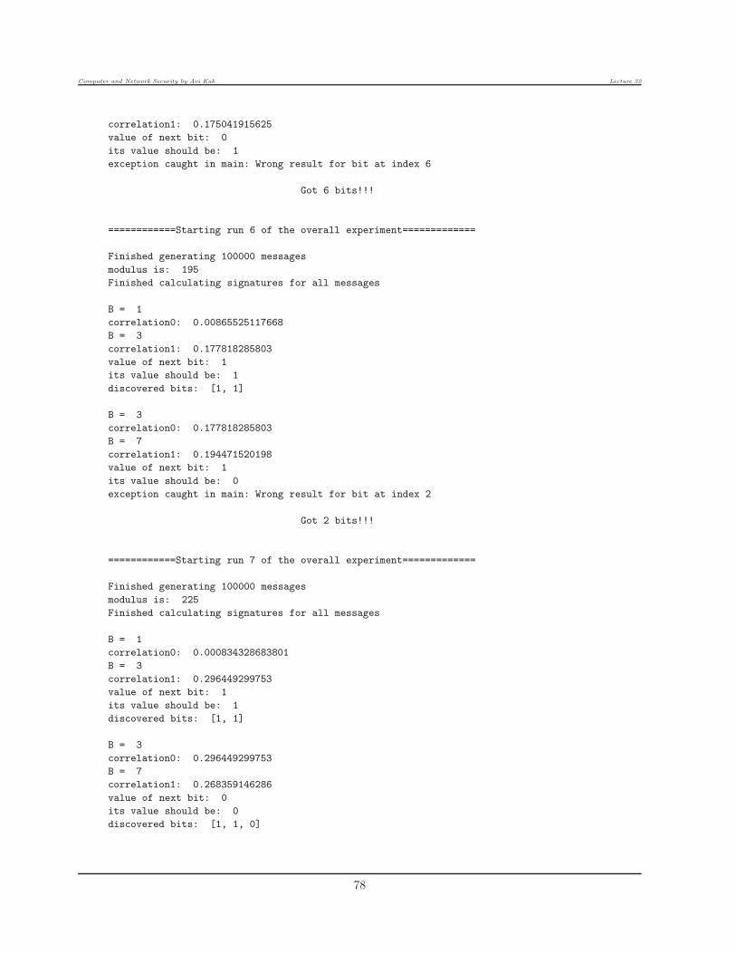
Computer and Network Security by Avi Kak Lecture 32
correlation1: 0.175041915625
value of next bit: 0
its value should be: 1
exception caught in main: Wrong result for bit at index 6
Got 6 bits!!!
============Starting run 6 of the overall experiment=============
Finished generating 100000 messages
modulus is: 195
Finished calculating signatures for all messages
B = 1
correlation0: 0.00865525117668
B = 3
correlation1: 0.177818285803
value of next bit: 1
its value should be: 1
discovered bits: [1, 1]
B = 3
correlation0: 0.177818285803
B = 7
correlation1: 0.194471520198
value of next bit: 1
its value should be: 0
exception caught in main: Wrong result for bit at index 2
Got 2 bits!!!
============Starting run 7 of the overall experiment=============
Finished generating 100000 messages
modulus is: 225
Finished calculating signatures for all messages
B = 1
correlation0: 0.000834328683801
B = 3
correlation1: 0.296449299753
value of next bit: 1
its value should be: 1
discovered bits: [1, 1]
B = 3
correlation0: 0.296449299753
B = 7
correlation1: 0.268359146286
value of next bit: 0
its value should be: 0
discovered bits: [1, 1, 0]
78

Computer and Network Security by Avi Kak Lecture 32
B = 3
correlation0: 0.296449299753
B = 11
correlation1: 0.200498385434
value of next bit: 0
its value should be: 1
exception caught in main: Wrong result for bit at index 3
Got 3 bits!!!
============Starting run 8 of the overall experiment=============
Finished generating 100000 messages
modulus is: 195
Finished calculating signatures for all messages
B = 1
correlation0: 0.0099350807053
B = 3
correlation1: 0.100855277594
value of next bit: 1
its value should be: 1
discovered bits: [1, 1]
B = 3
correlation0: 0.100855277594
B = 7
correlation1: 0.123326809251
value of next bit: 1
its value should be: 0
exception caught in main: Wrong result for bit at index 2
Got 2 bits!!!
============Starting run 9 of the overall experiment=============
Finished generating 100000 messages
modulus is: 225
Finished calculating signatures for all messages
B = 1
correlation0: -0.00389727670499
B = 3
correlation1: 0.251815183197
value of next bit: 1
its value should be: 1
discovered bits: [1, 1]
B = 3
correlation0: 0.251815183197
B = 7
correlation1: 0.224629240235
value of next bit: 0
79

Computer and Network Security by Avi Kak Lecture 32
its value should be: 0
discovered bits: [1, 1, 0]
B = 3
correlation0: 0.251815183197
B = 11
correlation1: 0.253504735599
value of next bit: 1
its value should be: 1
discovered bits: [1, 1, 0, 1]
B = 11
correlation0: 0.253504735599
B = 27
correlation1: 0.205049470386
value of next bit: 0
its value should be: 0
discovered bits: [1, 1, 0, 1, 0]
B = 11
correlation0: 0.253504735599
B = 43
correlation1: 0.186280401626
value of next bit: 0
its value should be: 0
discovered bits: [1, 1, 0, 1, 0, 0]
B = 11
correlation0: 0.253504735599
B = 75
correlation1: 0.195741658334
value of next bit: 0
its value should be: 1
exception caught in main: Wrong result for bit at index 6
Got 6 bits!!!
80

Computer and Network Security by Avi Kak Lecture 32
32.8: USB MEMORY STICKS AS ASOURCE OF DEADLY MALWARE
• Who could have imagined that the innocuous looking USB mem-
ory sticks would become be a potential source of deadly malware!
That this is indeed the case was demonstrated very convincingly
by Karsten Nohl and Jacob Lell at the 2014 Black Hat conference:
https://srlabs.de/blog/wp-content/uploads/2014/07/SRLabs-BadUSB-BlackHat-v1.pdf
This exploit was named BadUSB by its discoverers. It is esti-
mated that roughly half the USB devices out there are vulnerable
to the BadUSB exploit.
• If you do read the Nohl and Lell paper mentioned above, you
owe it your yourself to also go through the following report by
Stephanie Blanchet Hoareau, Erwan Le Disez, David Boucher,
and Benoit Poulo-Cazajou:
http://www.bertin-it.com/brochure/WP-BadUSB_an-unpatchable-flaw-by-Bertin-IT.pdf
One of the things I enjoyed about this well-written report is
the historical context it provides for the BadUSB exploit. It
was through this report I found out that, back in 2011, Ange-
los Stavrou and Zhaohui Wang gave a talk in that year’s Black
Hat conference that was entitled “Exploiting Smart-Phone USB
81

Computer and Network Security by Avi Kak Lecture 32
Connectivity For Fun And Profit,” in which they showed how an
Android phone connected to a computer as a USB device could
be emulated to act like a keyboard in order to inject hostile com-
mands into the host.
• It is important to realize that BadUSB is not about any mal-
ware files in the flash memory of a USB stick. [It is possible to detect those by
anti-virus software and, in the worst case, you can always just reformat a memory stick to get rid of any sus-
pected malware that resides in the flash memory of the stick.] BadUSB is about malware
threats that reside in the microcontroller firmware that con-
trols how the device operates. The current tools for detecting
malware are unable to identity these firmware based threats.
One can make the argument that the very nature of this malware
is such that it will not lend itself to detection by virus scanning
tools, present or future. See the end of this section for this ar-
gument. [BadUSB is also not about the “USB Propagation Mode” for malware that was described in
Lecture 22. As the reader will recall, if a Windows machine has “AutoRun” enabled, a file named autorun.inf
in the USB device would be automatically executed when the device is plugged into the computer. An infected
copy of this file in the device can infect a computer with the malware.]
• Karsten Nohl and Jacob Lell chose to not make public the soft-
ware for their exploit. That talk was followed by a presentation
entitled “Making BadUSB Work For You” at the Derbycon 2014
conference by Adam Caudill and Brandon Wilson where they
showed that they had successfully developed their own imple-
mentation of the BadUSB exploit. They have made their code
available on GitHub.
82

Computer and Network Security by Avi Kak Lecture 32
• Now that the cat is out of the bag and people have started posting
code on the web that makes this exploit possible, you may want
to exercise greater caution when you stick your memory stick in
other people’s computers or stick other people’s memory sticks
in your own. [When in a hotel, who hasn’t downloaded the boarding passes from an airline website
into a personal memory stick and taken the stick over to a hotel computer for printing them out! In light of
the BadUSB exploit, you may never want to do that again. (In the future, you may just want to download
the boarding pass into your smartphone directly). With all and sundry plugging their memory sticks into that
hotel computer in the lobby, there is always the possibility that, intentionally or unintentionally, someone may
use the BadUSB exploit to plant malware on that computer. Just imagine the consequence that after your own
memory stick has become infected in this manner, you plug it into your own computer!]
• To understand the BadUSB exploit, it’s best to revisit the main
reason the USB standard was created back in the mid 1990’s.
What prompted the development of this standard was the ever
increasing choice of peripherals that people could connect with
their computers: keyboard, mouse, webcam, music player, exter-
nal drive, and so on. It was felt that if a single connector type
could be devised for all such peripherals, that would considerably
simplify the hardware support that would need to be incorpo-
rated in a computer for the data transfer connections with the
different peripherals. [The USB standard has fulfilled that goal. The acronym USB stands for
”Universal Serial Bus”. One reason for the popularity of USB for connecting portable devices to a computer is
that you can connect and disconnect the devices without having to reboot the host computer. That is, USB
devices tend to be hot-swappable.]
• Considering that so many different types of devices can present
83

Computer and Network Security by Avi Kak Lecture 32
themselves to your computer through a USB connection, haven’t
you wondered as to how is it that a computer can tell the dif-
ference between, say, a keyboard and a thumb drive if they both
present themselves to your computer through the same hardware
port?
• When you insert a USB device in your computer, the very first
thing the OS in your computer does is to determine what “USB
class” the device belongs to. The USB standard defines a large
number of classes (over 20), some of the most commonly used
being:
Human Interface Device (HID) : USB devices that belong to this class are usedfor connecting pointing devices (computer mouse, joystick), keypads, keyboards,etc.
Image : USB devices that belong to this category are used for connecting webcam,scanner, etc., to a computer.
Printer : As you might guess from its name, USB devices that fall in this class areused to connect different types of printers to a computer.
Mass Storage (MSC) : USB devices that belong to this class are used for flash mem-ory drives, digital audio players, cameras, etc. [As you might have guessed already, the
acronym MSC stands for ”Mass Storage Class”. Another name for this class is UMS for ”USB Mass
Storage”.]
USB Hub : Such a device is used to expand a single USB port into several others.[Some of the lightest laptops come with only a single USB port. If you wanted to connect multiple devices
to such a laptop, you need a USB Hub. Also, when a machine does possess multiple USB ports, it is
usually an internally built single USB Hub that is expanded into multiple ports you see on the outside of
your laptop (rather than having independent USB circuitry for each separate port).]
84

Computer and Network Security by Avi Kak Lecture 32
Smart Card : These types of USB devices can be used to read smartcards.
and several others
• Each of the USB device classes is given a numerical code in the
USB standard. For example, the numerical code associated with
the HID class is 0x03, the code associated with the MSC class
0x08.
• As mentioned earlier, as soon as the OS on a host computer has
detected a USB device, it queries the USB device for the class
the device belongs to. The USB device responds back with the
numerical code of the class. The OS then loads the software
driver appropriate to that device class. [Subsequently, all communications between
the host computer and the USB device is in the form of packets. The first byte of each packet is the packet
identifier byte, which declares the purpose of the packet. For example, a packet may be a handshaking packet,
or a data bearing packet, or perhaps an error or a status message packet, etc.]
• Assuming the USB device is of class MSC, the software driver
in the host computer then interacts with the firmware in the
microcontroller in the USB device for transferring data between
the host computer and the flash memory in the USB memory
stick. [A microcontroller is just a small inexpensive single-chip computer, with its own CPU, RAM, and
I/O, that, for USB devices, is powered by the current drawn through the USB port from the host computer.
And the firmware consists of program stored in an EEPROM (Electrically Erasable Read Only Memory) that
is executed in the CPU of the microcontroller.]
85

Computer and Network Security by Avi Kak Lecture 32
• The ”mini-review” of USB devices presented so far describes how
such devices work under normal conditions. Let’s now consider
the following aspect of the firmware that sits in the microcon-
trollers of such devices that can turn a memory stick into a dan-
gerous source of malware.
• To allow for bug fixes to be carried out in the firmware in a USB
microcontroller and to also allow for the firmware to be upgraded,
the USB manufacturers permit third-party tools to alter their
firmware. In fact, you can download a manufacturer-consortium
supported open-source tool called ”USB Device Firmware Up-
grade tool” for this purpose from
https://admin.fedoraproject.org/pkgdb/package/dfu-util/
This is a vendor- and device-independent Device Firmware Up-
grade (DFU) tool for upgrading the firmware in the USB devices.
You can use this tool to both download the firmware currently in
the USB device and to upload to the device a new version of the
firmware.
• The fact that one can replace the manufacturer’s firmware in
the microcontroller of a USB opens it up to exploits for spread-
ing malware infection. Here is how that can happen: You take
a memory stick (that would normally belong to the class MCS)
and you alter its firmware so that, upon being inserted into a
host computer, it reports to the OS that its class is HID. That
would allow the USB stick to act as a keyboard vis-a-vis the host
86

Computer and Network Security by Avi Kak Lecture 32
computer it is connected to. Any keystrokes sent by the USB
masquerading as a keyboard could be for executing commands
that install malware from remote sites. The commands executed
in this manner could also install malware that would be perma-
nently stored in the host and installed in all USBs memory sticks
that are plugged into the host in the future.
• What makes this exploit particularly dangerous is that it is unde-
tectable by any virus scanning tools. These tools are not meant
for examining the firmware in the peripheral devices connected
to a computer.
• Obviously, your first reaction to the state of affairs described in
the previous bullet is likely to be: Why not augment the virus
scanning tools to also look at the firmware in the peripheral de-
vices connected to a host? You might think of a scanning tool
that is placed at the disposal of the OS so that when the OS first
detects a USB devices, it makes a point of examining the firmware
before allowing any data exchange with the device. However there
is a problem with that scenario: How would this tool distinguish
between a USB that belongs legitimately to the HID class and
the devices that are masquerading as belonging to the same?
87

Computer and Network Security by Avi Kak Lecture 32
32.9: MOBILE IP
• Let’s say you are at home and you want to use your smartphone
to send a text message to your friend who lives in the same town
as you, but who at the moment happens to be enjoying a local
brew in a Starbucks in a far-away country. Let’s assume that
your friend’s smartphone is connected to that Starbuck’s WiFi.
• The fact that your text message will reach your friend’s smart-
phone regardless of where exactly he/she is on the face of the
earth is pretty amazing. Haven’t you ever wondered how is it
that the cell phone operator at your end of the communication
link knows how to route your packets to your friend’s phone re-
gardless of the location of that phone? [The communication problem involved here
is more complex than you might think. In the old days, when all telephones had fixed numbers, a telephone
exchange at the source end of a communication link could immediately figure out how to route a phone call
just by examining the country code, the area code, etc., associated with a dialed number. But that obviously
does not apply to modern cell-phone based communications. You might think that a smartphone currently
connected to the internet in some remote country has an IP address assigned to it by the ISP in that remote
location. (That would certainly be the case for a non-mobile device like a laptop.) If that is indeed the case,
how would be network at the source end know how to route the packets to the remote phone if it is the source
that is initiating the connection?]
88

Computer and Network Security by Avi Kak Lecture 32
• The answer to the question posed above lies in the concept of
what is known as IP Mobility Support as defined in RFC 5944.
What RFC 5944 spells out is also informally referred to asMobile
IP.
• According to the RFC 5944 standard, every mobile “node” in a
network is always identified by its home IP address, regardless
of the current location of the node. When away from home, a
mobile node also has another IP address associated with it; this
second IP address is known as care-of IP address. [Think of the home
IP address as the permanent identifier for a smartphone. When a smartphone is away from its
home network, it needs both IP addresses, the home IP address and the care-of IP address, to
operate according to RFC 5944.]
• Whereas a mobile node is uniquely identified by its home IP ad-
dress, the care-of IP address, when it exists, is the mobile node’s
current point-of-attachment with the internet.
• Informally speaking, the cell phone operator where the home IP
address for a mobile node is registered is referred to as the home
agent in RFC 5944. And the cell phone operator at the mobile
node’s current point of attachment is known as the node’s foreign
agent. [For the official definitions: Home Agent: A router on a mobile node’s home network that
tunnels datagrams for delivery to the mobile node when it is away from home, and maintains current
location information for the mobile node. Foreign Agent: A router on a mobile node’s visited network
that provides routing services to the mobile node while registered. The foreign agent detunnels and
delivers to the mobile node datagrams that were tunneled by the mobile node’s home agent. For
89

Computer and Network Security by Avi Kak Lecture 32
datagrams sent by a mobile node, the foreign agent may serve as a default router for registered mobile
nodes.]
• Regardless of the current point of attachment for a mobile node,
if your smart phone wants to send packets to that mobile node,
it sends the packets to the mobile node’s home agent. The home
agent tunnels the packets to the mobile node’s current foreign
agent, which, in turn, routs the packets to their final destination
using the care-of IP address. This is illustrated by the following
diagram taken from RFC 5944:
2) Datagram is intercepted 3) Datagram is
by home agent and detunneled and
is tunneled to the delivered to the
care-of address. mobile node.
+-----+ +-------+ +------+
|home | =======> |foreign| ------> |mobile|
|agent| | agent | <------ | node |
+-----+ +-------+ +------+
1) Datagram to /|\ /
mobile node | / 4) For datagrams sent by the
arrives on | / mobile node, standard IP
home network | / routing delivers each to its
via standard | |_ destination. In this figure,
IP routing. +----+ the foreign agent is the
|host| mobile node’s default router.
+----+
Operation of Mobile IPv4 (from RFC 5944)
• In the diagram shown above, the “host” at the bottom of the
diagram could be your smart phone and the “mobile node” the
90
Computer and Network Security by Avi Kak Lecture 32
smart phone of your friend at any remote location on earth where
there is cell phone coverage.
• What’s most interesting about the routing diagram shown above
is the path taken by the packets from the remote cell phone back
to your smart phone. As shown by the diagonal arrow, the return
path for the packets bypasses the home agent.
• Another important point related to the return packets is that
source IP address in those packets is the mobile node’s home IP
address. So as far as the “host” at the bottom of the diagram
is concerned, the packets it receives from the remotely located
mobile node look as if the mobile node were located in its home
network.
• Let’s get back to the subject of your smartphone sending packets
to your friend’s smartphone that is currently at a remote loca-
tion. The data coming off your smartphone will look no different
from when your friend phone is plugged into the home network.
It is the job of the router in the home network to tunnel the
packets coming off your phone to the router at the current point
of attachment of your friend’s phone. Tunneling means that the
home router places the packets coming off your smartphone in
the data payload of the packets sent to the router where your
friend’s smartphone is currently located. That router detunnels
the packets and sends them to your friend’s smartphone.
91