Lecture 30

Line integrals of vector fields over closed curves

(Relevant section from Stewart, Calculus, Early Transcendentals, Sixth Edition: 16.3)

Recall the basic idea of the Generalized Fundamental Theorem of Calculus: If F is a gradient or

conservative vector field – here, we’ll simply use the fact that it is a gradient field, i.e., F = ~∇f for

some f – and C is a curve that starts at point A and ends at point B, then

∫

CF · dr =

∫

C

~∇f · dr (1)

= f(B) − f(A).

In other words, the line integral, which could represent the work done by F if a particle is moved from

A to B, depends only on the endpoints A and B and not on the curve from A to B.

Now we consider the following question: What if curve C started at A, travelled around for a

while and then ended back at A – in other words, A = B? Of course, this means that f(B) = f(A),

which would imply that the line integral is zero. You’ve already encountered such situations in your

elementary mechanics course: Suppose that you start with an object lying on a table, pick it up, walk

around with it, perhaps going down the stairs, out the building, etc., then enter the building again,

come back to the table and place the object on it. If we employ the approximation that the potential

energy of the object is V (y) = mgy, where, for convenience, y = 0 is the table surface, then the net

change in potential energy ∆V = 0, so no net work was done by gravity.

In physics and other applications, one is often concerned with line integrals of vector fields over

simple, closed curves C. “Simple” means nonintersecting. “Closed” means that the curve has no

endpoints – you pick any starting point on the curve and you’ll eventually arrive back at it. Such line

integrals are often denoted as follows∮

CF · dr. (2)

One would be tempted to conclude that line integrals of conservative vector fields over closed curves

are always zero since we end up where we started from. This is, in fact, often the case. But there

are situations in which it is not zero. The problem is that we have to revise slightly our definition

of a conservative field, paying attention to the region D over which we perform the integration. If

this region contains singularities of the vector field F, i.e., points at which F or its derivatives do

223

not exist, then line integrals of “supposedly conservative” vector fields F over closed curves are not

necessarily zero. It is possible that these singularities will “interfere” with line integrals over curves

that “enclose” them. We’ll explain below.

It’s convenient to consider two cases. In both cases, we let D denote a region of interest in Rn

over which we wish to consider line integrals of a vector field F. We shall also let C denote a simple,

closed curve that lies entirely in D, also assuming that it is piecewise smooth, so that the line integral

may be computed (we need the tangent r′(t) to be defined):

1. The “nice” case: Suppose that F and its derivatives are defined at all points in D. Further-

more, suppose that

curl F(r) = ~∇× F(r) = 0 at all points r ∈ D. (3)

Then F is conservative on D and the line integral

∮

CF · dr = 0 (4)

over any simple curve D.

We have already encountered a number of examples for this case. For example, a couple of

lectures ago, we examined the vector field,

F(x, y) = 2x i + 4y j + z k, (5)

It is conservative, since Eq. (3) is satisfied at all points in R3. We also found that F = ~∇f ,

where

f(x, y, z) = x2 + 2y2 +1

2z2. (6)

F and its derivatives are defined at all points in R3. Therefore Eq. (4) holds for any closed

curve C in any region D ⊂ R3.

2. The “not-so-nice” case: Suppose that F and/or its derivatives are undefined at some points

in D – we refer to such points as singularities. At all other points in D, we assume that

curl F(r) = ~∇× F(r) = 0. (7)

Sub-case No. 2(a): Consider the situation sketched in the figure below. Here, we are looking

at a simple closed curve C in the plane. The point P is a singularity of the vector field F. At

all other points (x, y), we assume that Eq. (7) holds.

224

Clearly, the curve C does not enclose the singularity P , so we suspect that it can “avoid” this

singularity. Just to be a little more mathematical, take any point on C – call it point A. Then

start shrinking the curve C continuously to point A, keeping it fixed, as sketched in the figure.

If you can perform this shrinking operation until you end up at the single point A without

passing through a singularity, then the original line integral of F over the original curve C

is zero, i.e., Eq. (4) holds. In the figure below, this can be done – in other words, the singularity

P can be avoided.

A

C

y

x

P.

The singularity P can be avoided duringthe shrinking of curve C

(singularity)

Therefore, line integral is zero

Sub-case No. 2(b): In the next figure, we consider another curve C which now encloses the

singularity P . P . In this situation, we cannot shrink the curve C to point A without crossing

the singularity P . In this case, the line integral of F over the curve C is not necessarily zero

even though the curl of the vector field F is zero everywhere else. Unfortunately, that is all that

we can conclude – we would actually have to compute the line integral in some way in order to

see if it is zero or not.

y

x

.

the shrinking of curve C

C

A

The singularity P cannot be avoided during

Therefore, line integral is not necessarily zero

P

225

In the above examples, we were concerned with singularities of planar vector fields, i.e., vector

fields in R2. Clearly, if a simple curve C encloses a singular point P , there is no way that we

can avoid this singularity as the curve C is shrunk toward any point A on the curve.

Sub-case No. 2(c): On the other hand, if a vector field F in 3-space, i.e., R3 has a singular

point P , you can imagine that it can be avoided as we shrink a closed curve C. For example,

suppose that the singular point P is on the xy-plane, and suppose that our closed curve C is

also on the xy-plane, as sketched below. As we shrink the curve C toward a point A, we are

allowed to “lift” it up to avoid P during the process. In this case, the line integral of F over the

original curve is zero - assuming, of course, that ~∇× F = 0 at all other points.

In this sense, the space R3 is more “forgiving.” For this reason, we may state that the grav-

itational force F due to a point mass M at the origin is conservative, even though it has a

singularity at (0, 0, 0): The line integral of F over any closed curve C, provided that C does not

contain the singular point (0, 0, 0) is zero.

.

A

P

C

In R3, the singularity at P can be avoided by deforming

or “lifting” the curve C as it is being shrunk toward A

Sub-case No. 2(d): But the space R3 is not totally forgiving! Suppose that we have a vector

field – and we’ll consider a physically meaningful one in a few moments – that has a line of

singularities, for example, on the z-axis. At all other points, ~∇ × F = 0. Then, as sketched

below, it is impossible for any curve C that encloses the z-axis to be shrunk to a point without

crossing the z-axis. Therefore, no conclusions can be made about the line integral of F over C.

On the other hand, any curve C ′ that does not enclose the z-axis can be deformed to a single

point, implying that the line integral of F over C ′ is zero.

226

C

C′

line of singularities on z-axis

In R3, the singularities on the z-axis cannot be avoided by deforming

the curve C as it is being shrunk toward A

A

On the other hand, curve C′ can be shrunk to a point

Connected and simply connected sets

A compact mathematical summary of the above cases can be made in terms of connected and

simply connected sets. In the “nice” case above, where there are no singularities, we are working

with simply connected sets – it is possible to shrink closed curves to single points without leaving the

set. On the other hand, in the “not-so-nice” case, the singularities of the vector field, where it is not

defined, represent “missing” points. In such cases, closed curves cannot be shrunk to single points

without leaving the set. The set is then not simply connected. Some additional comments on these

definitions are presented in an Appendix at the end of this lecture. (The material in the Appendix

was not presented in class, and is to be considered as supplementary material.)

We now illustrate with an example. Consider the following vector field in R2:

F(x, y) =

(

−y

x2 + y2,

x

x2 + y2

)

. (8)

Note that F(0, 0) is undefined. In a recent Problem Set, you showed that ~∇ × F = 0 at all points

except (0, 0), where it is undefined. Let’s review this calculation:

~∇× F =

∣

∣

∣

∣

∣

∣

∣

∣

∣

i j k

∂/∂x ∂/∂y ∂/∂z

−y/(x2 + y2) x/(x2 + y2) 0

∣

∣

∣

∣

∣

∣

∣

∣

∣

= 0i + 0j +

(

∂

∂x

[

x

x2 + y2

]

−∂

∂y

[

−y

x2 + y2

])

k

= 0i + 0j +

(

1

x2 + y2−

2x2

(x2 + y2)2+

1

x2 + y2−

2y2

(x2 + y2)2

)

k

= 0i + 0j + 0k, (x, y) 6= (0, 0).

227

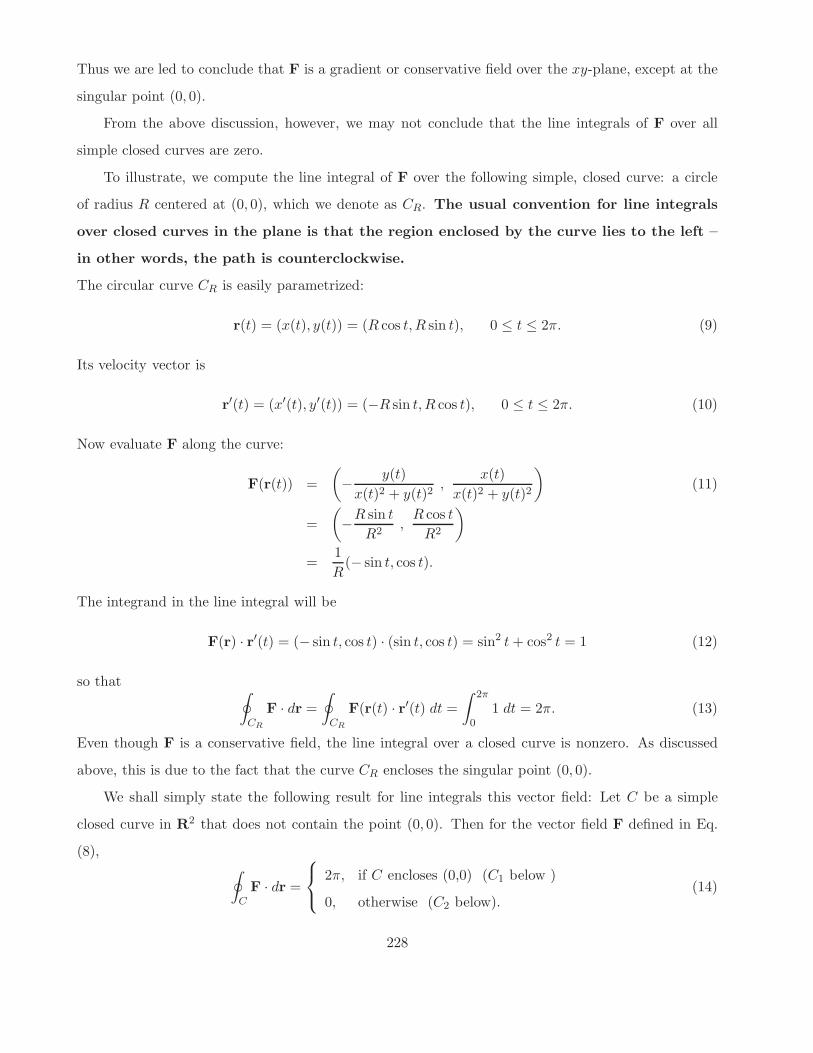
Thus we are led to conclude that F is a gradient or conservative field over the xy-plane, except at the

singular point (0, 0).

From the above discussion, however, we may not conclude that the line integrals of F over all

simple closed curves are zero.

To illustrate, we compute the line integral of F over the following simple, closed curve: a circle

of radius R centered at (0, 0), which we denote as CR. The usual convention for line integrals

over closed curves in the plane is that the region enclosed by the curve lies to the left –

in other words, the path is counterclockwise.

The circular curve CR is easily parametrized:

r(t) = (x(t), y(t)) = (R cos t, R sin t), 0 ≤ t ≤ 2π. (9)

Its velocity vector is

r′(t) = (x′(t), y′(t)) = (−R sin t, R cos t), 0 ≤ t ≤ 2π. (10)

Now evaluate F along the curve:

F(r(t)) =

(

−y(t)

x(t)2 + y(t)2,

x(t)

x(t)2 + y(t)2

)

(11)

=

(

−R sin t

R2,

R cos t

R2

)

=1

R(− sin t, cos t).

The integrand in the line integral will be

F(r) · r′(t) = (− sin t, cos t) · (sin t, cos t) = sin2 t + cos2 t = 1 (12)

so that∮

CR

F · dr =

∮

CR

F(r(t) · r′(t) dt =

∫ 2π

01 dt = 2π. (13)

Even though F is a conservative field, the line integral over a closed curve is nonzero. As discussed

above, this is due to the fact that the curve CR encloses the singular point (0, 0).

We shall simply state the following result for line integrals this vector field: Let C be a simple

closed curve in R2 that does not contain the point (0, 0). Then for the vector field F defined in Eq.

(8),∮

CF · dr =

2π, if C encloses (0,0) (C1 below )

0, otherwise (C2 below).(14)

228

O

C1

C2

x

y

For reasons that will become clear in the next lecture, let us now consider the above vector field

as a field in R3, i.e.,

F(x, y, z) = −y

x2 + y2i +

x

x2 + y2j + 0 k. (15)

In other words, we simply translate this vector field upwards and downwards from the xy-plane into

R3.

We have now produced a vector field in R3 that has a line of singularities along the z-axis. We

now have the situation pictured in Sub-case No. 2(d) above. The final result is the following: For a

simple, closed curve C in R3 that does not contain any points from the z-axis,

∮

CF · dr =

2π, if C encloses the z axis

0, otherwise.(16)

229

Appendix: Connected and simply connected sets (not covered in lecture)

The above discussion can be phrased in more mathematical language as follows. For the line integral

∫

CF · dr (17)

to be independent of path, which includes the consequence that

∮

CF · dr = 0, (18)

where C is a closed curve, we must have that ~∇× F = 0 over a simply connected set, or at least the

region of interest D, over which all integrations are being performed, is a simply connected set. Of

course, we now have to define “simply connected.”

Connected and simply connected sets

Let U ⊆ Rn. Then U is said to be connected if any two points P,Q ∈ U can be joined by a continuous

curve C that is contained entirely in U – in other words, all points of C are contained in U .

A set U is connected if it is “in one piece.”

Examples: (Verify these results with your own sketches.)

1. The sets R, R2 and R3 are simply connected.

2. The set R−{0}, also written as R\{0}, which is obtained by removing the point x = 0 from the

real line, is not simply connected: It consists of two disconnected pieces, (−∞, 0) and (0,∞).

You can’t connect a point P to the left of 0 to a point Q to the right of 0 with a continuous

“curve”, in this case a line segment, without going through 0, which is not part of the set.

3. The set R2{(0, 0} is connected.

230

4. On the other hand, the set R2 − {y-axis} is not connected – the plane is separated into two

disconnected sets, x > 0 and x < 0

5. The set R2 − { the circle x2 + y2 = 1} is not connected. Taking away this circle leaves two

disconnected sets – the interior of the circle and the exterior.

6. The set R3 − {(0, 0, 0)} is connected.

7. The set R3 − { z-axis } is connected.

8. The set R3 − { the plane z = 0} is not connected.

A set U ∈ Rn is simply connected if it is connected and if every simple closed curve in U can be

continuously shrunk to a point in U without leaving the set. A simply connected set in R2 cannot

have holes.

Examples: (Once again, verify these results with your own sketches.)

1. The sets R, R2 and R3 are simply connected.

2. The set R2\{(0, 0)}, obtained by removing the point (0, 0) from R2 is not simply connected.

3. The set R3\{(0, 0, 0)}, obtained by removing the point (0, 0, 0) from R3 is simply connected.

(You can avoid the origin when you shrink any curve.)

4. The set {(x, y, z) ∈ R3 | (x, y) 6= (0, 0)}, the set obtained by removing the z-axis from R3, is not

simply connected. Any closed curve that encloses the z-axis cannot be shrunk to a point without

leaving the set, i.e., crossing the z-axis. This example will be important in an application to

physics that we shall study in the next lecture.

231

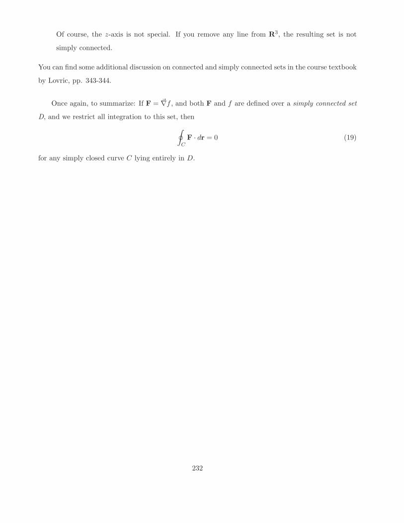
Of course, the z-axis is not special. If you remove any line from R3, the resulting set is not

simply connected.

You can find some additional discussion on connected and simply connected sets in the course textbook

by Lovric, pp. 343-344.

Once again, to summarize: If F = ~∇f , and both F and f are defined over a simply connected set

D, and we restrict all integration to this set, then

∮

CF · dr = 0 (19)

for any simply closed curve C lying entirely in D.

232

Lecture 31

Line integrals of vector-valued functions (cont’d)

Circulation of a vector field around a closed curve C in R2

In what follows, we consider the line integral of a planar vector field F around a simple closed curve C

in R2. The convention is that the integration along C is performed in the counterclockwise direction

so that the region D enclosed by C lies always to the left of C as we move along the curve. Let’s recall

that this line integral sums up the projection of the vector field onto the unit tangent vector T to the

curve. Assuming that we can parametrize this curve as r(t), a ≤ t ≤ b,

∮

CF · ds =

∫ b

aF(r)(t)) · r′(t) dt (20)

=

∫ b

aF(r)(t)) ·

r′(t)

‖ r′(t) ‖‖ r′(t) ‖ dt

=

∫ b

aF(r)(t)) · T(t) ds

=

∮

fds,

where the scalar-valued function f(r(t)) = F(r(t)) · T(t) is the projection of F in the direction of the

unit tangent vector to the curve C at r(t):

CT(t1)

T(t2)

T(t3)

F(x(t3)

T(t4)

F(x(t4))

F(x(t1))

F(x(t2))

Starting at any point P on the curve C, the orientation of the tangent vector T will change as we

travel along C. In one traversal of C, the net rotation of the tangent vector is 2π. This is quite clear

when C is a circle. As such, we say that the line integral in (20) is the circulation of the vector field

F around the closed curve C.

If the vector field F is roughly parallel over the region D enclosed by curve C, then we expect the

line integral to be small in value – in some regions of the curve, F points in the same direction as T

and in others, it points in the opposite direction. In other words, the vector field exhibits very little

233

circulation.

Example 1: Let’s consider a very simple case:

F(x, y) = K i (21)

and C = CR is the circle of radius R centered at the origin:

F = Ki

y

x

CR

RO

1. Parametrization of curve CR: r(t) = (R cos t, R sin t), 0 ≤ t ≤ 2π.

2. Velocity: r′(t) = (−R sin t, R cos t).

3. Evaluate F on curve: F(r(t)) = (K, 0).

4. Integrand: F(r(t)) · r′(t) = (K, 0) · (−R sin t, R cos t) = −KR sin t.

Thus∮

CR

F · ds = −KR

∫ 2π

0sin t dt = 0. (22)

As expected, the line integral is zero.

Example 2: Here is another situation that we expect will produce a zero result: C = CR as before

and

F(x, y) = Kr = Kxi + Kyj (23)

In this case, the vector F on the curve is perpendicular to the tangent vector:

1. Parametrization of curve CR: r(t) = (R cos t, R sin t), 0 ≤ t ≤ 2π.

2. Velocity: r′(t) = (−R sin t, R cos t).

234

$x$

$y$

$0$ $R$

$C_R$

F = Kr

3. Evaluate F on curve: F(r(t)) = K(x, y) = K(R cos t, R sin t).

4. Integrand: F(r(t))·r′(t) = K(R cos t, R sin t)·(−R sin t, R cos t) = −KR cos t sin t+KR cos t sin t =

0.

Thus∮

CR

F · ds =

∫ 2π

00 dt = 0. (24)

As expected, the line integral is zero.

Example 3: Now consider the vector field

F(x, y) = K(−yi + xj) (25)

as sketched below.

$R$$x$

$y$

$C_R$

$0$

You will recall that this is the velocity vector field of a disk that is revolving about the origin with

angular speed ω = K. In this case, F points in the direction of the unit tangent vector T at every

point on the curve CR. As such, we expect a nonzero result:

1. Parametrization of curve CR: r(t) = (R cos t, R sin t), 0 ≤ t ≤ 2π.

235

2. Velocity: r′(t) = (−R sin t, R cos t).

3. Evaluate F on curve: F(r(t)) = K(−y, x) = K(−R sin t, R cos t).

4. Integrand: F(r(t))·r′(t) = K(−R sin t, R cos t)·(−R sin t, R cos t) = KR2 sin t sin t+KR cos t cos t =

KR.

Thus∮

CR

F · ds =

∫ 2π

0KR2 dt = 2πKR2. (26)

As expected, the line integral is nonzero.

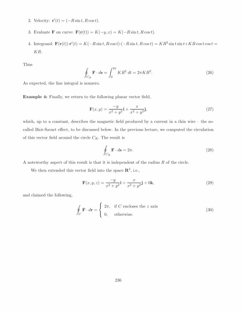
Example 4: Finally, we return to the following planar vector field,

F(x, y) =−y

x2 + y2i +

x

x2 + y2j, (27)

which, up to a constant, describes the magnetic field produced by a current in a thin wire – the so-

called Biot-Savart effect, to be discussed below. In the previous lecture, we computed the circulation

of this vector field around the circle CR. The result is

∮

CR

F · ds = 2π. (28)

A noteworthy aspect of this result is that it is independent of the radius R of the circle.

We then extended this vector field into the space R3, i.e.,

F(x, y, z) =−y

x2 + y2i +

x

x2 + y2j + 0k, (29)

and claimed the following,

∮

CF · dr =

2π, if C encloses the z axis

0, otherwise.(30)

236

Application to Physics: The Biot-Savart effect

The vector field of Example 4 above is important in electromagnetism as we now show. We are

concerned with the Biot-Savart effect, in which a current of charge flowing in a conducting wire

creates a magnetic field surrounding the wire.

In what follows, we assume that the conductor is a straight, thin wire such that the direction

of current is given by the unit vector u. The current vector is then given by I = Iu. The physical

situation is sketched below: P is a point of observation with position vector r.

of currentu direction vector

wire carrying electric current IO

P

r

B(r)

created by current I = Iumagnetic field B(r)

θ

A rough sketch of B was given in the handout sheets from Lecture 1. Here are three physical facts

that are verified by experiment (remember that Physics is an experimental science!):

1. The strength of the magnetic field ‖ B ‖ is proportional to the magnitude I of the current.

2. The strength of the magnetic field ‖ B ‖ diminishes as we move away from the wire. In fact, it

diminishes as 1/d, where d is the distance from the point of measurement P to the wire.

3. The magnetic field vector B(r) points in a direction that is perpendicular to the current vector

I. In fact, flow lines of the magnetic field are circles that lie on planes perpendicular to I.

From electrodynamics, the magnetic field at P is given by

B(r) =µ0I

2π

u × r

‖ u× r ‖2. (31)

Here, µ0 denotes the permeability of the vacuum. This equation accounts for the experimental obser-

237

vations given above. Note that

‖ B(r) ‖ =µ0I

2π

‖ u × r ‖

‖ u× r ‖2(32)

=µ0I

2π

1

‖ u× r ‖

=µ0I

2π

1

‖ r ‖ sin θ

=µ0I

2π

1

d,

where d = r sin θ is the distance from point P to the wire. We see that the strength of the magnetic

field decreases with the distance d and not with the square of the distance.

It is convenient to orient the coordinate system so that the wire lies on the z-axis, i.e. u = k.

Then the current vector I = Ik. The magnetic field vector then becomes

B(r) =µ0I

2π

k× r

‖ k× r ‖2. (33)

We compute the numerator:

k× r =

∣

∣

∣

∣

∣

∣

∣

∣

∣

i j k

0 0 1

x y z

∣

∣

∣

∣

∣

∣

∣

∣

∣

(34)

= −yi + xj

This means that ‖ k × r ‖2= x2 + y2 so that

B(r) =µ0I

2π

[

−y

x2 + y2i +

x

x2 + y2i + 0k

]

, (35)

which is the vector field of Example 4 above. Note that B is undefined for (x, y) = (0, 0), i.e. the

z-axis, which is the location of the current-carrying wire. This means that B(r) is defined on a set

that is not simply connected. If CR denotes the circle x2 + y2 = R2, independent of z, then

∮

CR

B · dr =µ0I

2π2π = µ0I. (36)

This is the circulation of the magnetic field over the circle CR. Note that it is independent of R. As

we move away from the wire, the strength of the magnetic field B decreases linearly with R. But the

238

length of the closed curve CR, its circumference, increases linearly with R. These two effects cancel

each other in the line integral, which accounts for the independence of R.

Let us recall that the magnetic vector field B is, apart from a constant, identical in form to the

example studied in the previous lecture. We have

~∇× B(r) = 0, (x, y) 6= (0, 0). (37)

In other words B is defined on the set obtained by removing the z-axis from R3, which is not simply

connected. On the other hand, any connected set in R3 that does not contain the z-axis is simply

connected. As a result, we have the following:

∮

CB · dr =

µ0I, if C encircles the z axis,

0, otherwise.(38)

239

Lecture 32

Line integrals of vector fields over closed curves (cont’d)

Outward flux of a vector field across a closed curve C in R2

We now return to the line integral in Eq. (20) of the previous lecture, replacing the unit tangent

vector T with the unit outward normal N to the curve C. This is the unit vector at a point r(t) on

the curve which is perpendicular to the unit tangent vector T(t) and which points outward from the

region D enclosed by C, as shown below:

n(t4)

F(x(t3)

C

n(t3)

F(x(t4))

F(x(t1))

F(x(t2))

n(t1)

n(t2)

The result is the line integral that we denote as

∮

CF · N ds =

∫ b

aF(r(t)) · N(t) ‖ r′(t) ‖ dt. (39)

Clearly, this line integral adds up the projection of the vector field F onto the outward normal along

the curve C. The result is the total outward flux of F across the closed curve C. If F represents the

velocity field of a fluid, then the total outward flux measures the net rate of fluid escape from the

region D through the curve C per unit time.

The practical calculation of the outward flux integral is not difficult – the only complication is

that you have to determine the outward unit normal vector N(t) to the curve C. This is easily done

from a knowledge of the velocity vector r′(t). You first construct the unit tangent vector as follows:

T(t) =1

‖ r′(t) ‖r′(t) = (T1(t), T2(t)). (40)

Note that T 21 + T 2

2 = 1. There are two unit vectors that are perpendicular to T(t) – we’ll define them

as

N1 = (T2(t),−T1(t)), N2 = −(T2(t),−T1(t)). (41)

240

We choose the vector that points outward.

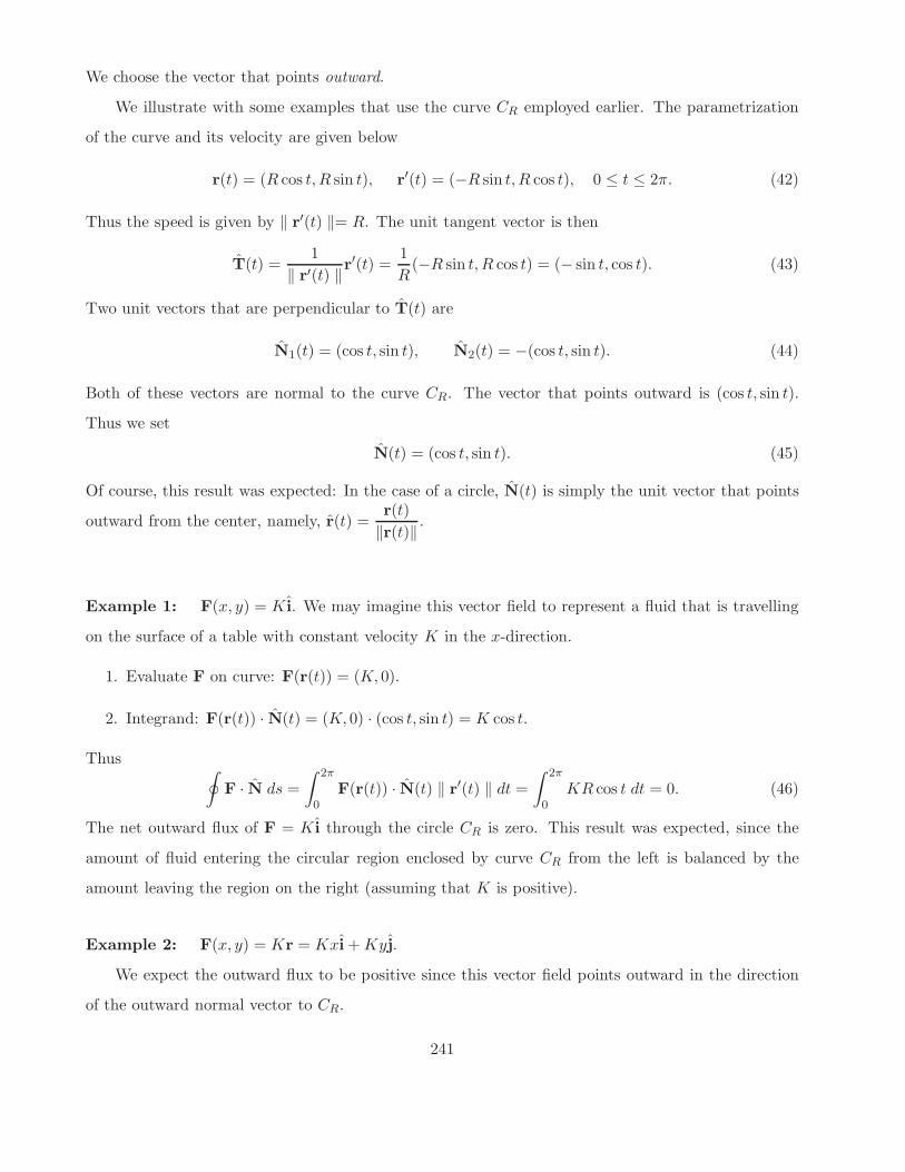
We illustrate with some examples that use the curve CR employed earlier. The parametrization

of the curve and its velocity are given below

r(t) = (R cos t, R sin t), r′(t) = (−R sin t, R cos t), 0 ≤ t ≤ 2π. (42)

Thus the speed is given by ‖ r′(t) ‖= R. The unit tangent vector is then

T(t) =1

‖ r′(t) ‖r′(t) =

1

R(−R sin t, R cos t) = (− sin t, cos t). (43)

Two unit vectors that are perpendicular to T(t) are

N1(t) = (cos t, sin t), N2(t) = −(cos t, sin t). (44)

Both of these vectors are normal to the curve CR. The vector that points outward is (cos t, sin t).

Thus we set

N(t) = (cos t, sin t). (45)

Of course, this result was expected: In the case of a circle, N(t) is simply the unit vector that points

outward from the center, namely, r(t) =r(t)

‖r(t)‖.

Example 1: F(x, y) = K i. We may imagine this vector field to represent a fluid that is travelling

on the surface of a table with constant velocity K in the x-direction.

1. Evaluate F on curve: F(r(t)) = (K, 0).

2. Integrand: F(r(t)) · N(t) = (K, 0) · (cos t, sin t) = K cos t.

Thus∮

F · N ds =

∫ 2π

0F(r(t)) · N(t) ‖ r′(t) ‖ dt =

∫ 2π

0KR cos t dt = 0. (46)

The net outward flux of F = K i through the circle CR is zero. This result was expected, since the

amount of fluid entering the circular region enclosed by curve CR from the left is balanced by the

amount leaving the region on the right (assuming that K is positive).

Example 2: F(x, y) = Kr = Kxi + Kyj.

We expect the outward flux to be positive since this vector field points outward in the direction

of the outward normal vector to CR.

241

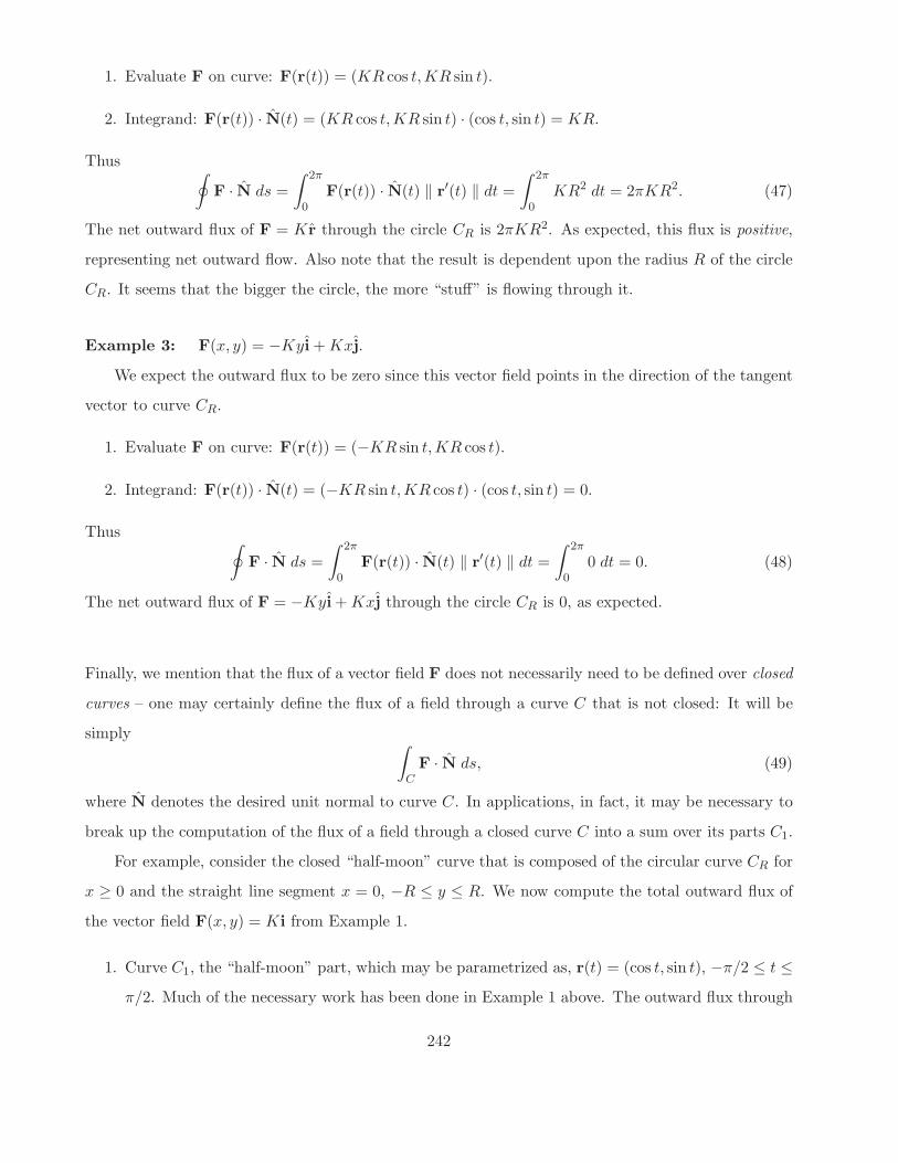
1. Evaluate F on curve: F(r(t)) = (KR cos t,KR sin t).

2. Integrand: F(r(t)) · N(t) = (KR cos t,KR sin t) · (cos t, sin t) = KR.

Thus∮

F · N ds =

∫ 2π

0F(r(t)) · N(t) ‖ r′(t) ‖ dt =

∫ 2π

0KR2 dt = 2πKR2. (47)

The net outward flux of F = K r through the circle CR is 2πKR2. As expected, this flux is positive,

representing net outward flow. Also note that the result is dependent upon the radius R of the circle

CR. It seems that the bigger the circle, the more “stuff” is flowing through it.

Example 3: F(x, y) = −Kyi + Kxj.

We expect the outward flux to be zero since this vector field points in the direction of the tangent

vector to curve CR.

1. Evaluate F on curve: F(r(t)) = (−KR sin t,KR cos t).

2. Integrand: F(r(t)) · N(t) = (−KR sin t,KR cos t) · (cos t, sin t) = 0.

Thus∮

F · N ds =

∫ 2π

0F(r(t)) · N(t) ‖ r′(t) ‖ dt =

∫ 2π

00 dt = 0. (48)

The net outward flux of F = −Kyi + Kxj through the circle CR is 0, as expected.

Finally, we mention that the flux of a vector field F does not necessarily need to be defined over closed

curves – one may certainly define the flux of a field through a curve C that is not closed: It will be

simply∫

CF · N ds, (49)

where N denotes the desired unit normal to curve C. In applications, in fact, it may be necessary to

break up the computation of the flux of a field through a closed curve C into a sum over its parts C1.

For example, consider the closed “half-moon” curve that is composed of the circular curve CR for

x ≥ 0 and the straight line segment x = 0, −R ≤ y ≤ R. We now compute the total outward flux of

the vector field F(x, y) = Ki from Example 1.

1. Curve C1, the “half-moon” part, which may be parametrized as, r(t) = (cos t, sin t), −π/2 ≤ t ≤

π/2. Much of the necessary work has been done in Example 1 above. The outward flux through

242

F = Ki

C1

−R

R

Rx

y

C2

C1 will be

∫

C1

F · N ds =

∫ 2π

0F(r(t)) · N(t) ‖ r′(t) ‖ dt =

∫ π/2

−π/2KR cos t dt = 2KR. (50)

This is the flux of the vector field through the curve C1.

2. Curve C2, the segment −R ≤ y ≤ R on the y-axis. Technically, we should compute this line

integral from the point y = R to y = −R so that we continue in a counterclockwise manner

on the boundary of the half-moon region. We cannot, however, simply parametrize the curve

as x(t) = 0, y(t) = t, R ≥ t ≥ −R, since t will then be decreasing over the integration. The

parameter must always be increasing in the integration, in order for the differential dt to be

positive. We thus parametrize the curve as x(t) = 0, y(t) = R − t, 0 ≤ t ≤ 2R. In other words

r(t) = (0, R − t), so that r′(t) = (0,−1) and ‖r′(t)‖ = 1.

The outward normal to this curve is the vector N = −i = (−1, 0). The integrand of the flux

integral will then be

F(r(t)) · N(t) = (K, 0) · (−1, 0) = −K. (51)

The flux across curve C2 will then be

∫

C2

F(r(t)) · N(t)‖r′(t)‖ dt =

∫ 2R

0−K dt = −2KR. (52)

Therefore the net outward flux through the half-moon region bounded by curves C1 and C2 is

∮

CF · N ds = 2KR − 2KR = 0. (53)

243

Classical Integration Theorems in the Plane

In this section, we present two very important results on integration over closed curves in the plane,

namely, Green’s Theorem and the Divergence Theorem, as a prelude to their important counterparts in

R3 involving surface integrals. Because of the lack of time in the lecture, the theorems were presented

very quickly. Examples will be presented in the next lecture.

Green’s Theorem in the Plane

(Relevant section from Stewart, Calculus, Early Transcendentals, Sixth Edition: 16.4)

Let F(x, y) = F1(x, y) i + F2(x, y) j be a vector field in R2. Let C be a simple closed (piecewise C1)

curve in R2 that encloses a simply connected (i.e., “no holes”) region D ⊂ R. Also assume that the

partial derivatives∂F2

∂xand

∂F1

∂yexist at all points (x, y) ∈ D. Then,

∮

CF · dr =

∫ ∫

D

[

∂F2

∂x−

∂F1

∂y

]

dA, (54)

where the line integration is performed over C in a counterclockwise direction, with D lying to the

left of the path.

Note:

1. The integral on the left is a line integral – the circulation of the vector field F over the closed

curve C.

2. The integral on the right is a double integral over the region D enclosed by C.

The Divergence Theorem in the Plane

This theorem is discussed in Section 16.4 of the text by Stewart, p. 1067, but only as a special case

of Green’s Theorem. Unfortunately, its important physical interpretation is not discussed in the text.

Let F(x, y) = F1(x, y) i + F2(x, y) j be a vector field in the plane. Let C be a simple closed

(piecewise C1) curve that encloses a region D. Let N denote the unit outward normal to C assumed

to exist at all points on the curve (except perhaps at a finite set of “corners”). Furthermore, assume

that the divergence of F is defined for all points in D, i.e.,

div F(x, y) = ~∇ · F(x, y) =∂F1

∂x(x, y) +

∂F2

∂y(x, y) (55)

244

is defined for all (x, y) ∈ D.

The Divergence Theorem in the Plane then states that

∮

CF · N ds =

∫ ∫

Ddiv F dA. (56)

The left integral is a line integral around the curve C – it measures the net outward flux of the vector

field F through the closed curve C. The right integral is a double integration over the region D

enclosed by C.

245