Lecture -- 3 -- Start - University of Pittsburghsuper7/51011-52001/51381.pdf · Lecture # 3:...

Lecture -- 3 -- Start

Outline

1. Science, Method & Measurement2. On Building An Index3. Correlation & Causality4. Probability & Statistics5. Samples & Surveys6. Experimental & Quasi-experimental Designs7. Conceptual Models8. Quantitative Models9. Complexity & Chaos10. Recapitulation - Envoi

Quantitative Techniques for Social Science Research

Ismail SerageldinAlexandria

2012

Lecture # 3:Correlation and Causality

No Textbooks? No handouts?

Again, there are so many text books covering this material…

Just THINK and follow the presentation.

Organizing Data

Data

Information

Knowledge

Wisdom

So

• We usually map (or plot) the data to be able to see it more clearly

• We try to link variables (making tables or graphs)

• We then try to find patterns or anomalies and try to interpret them.

Simple Table & Chi-Square

The most basic type of question

• Before we start, we expect (based on our hypothesis) that outcomes should be (e)

• Then we go and observe reality and find that outcomes are (o )

• So is the deviation (o - e) pure chance? or is it something else?

Chi Square

Chi-Square

• Chi-square is a statistical test commonly used to compare observed data (o) with data we would expect (e) to obtain according to a specific hypothesis.

• For example , based on Mendel’s laws, we expect that in a cross between pure green (dominant) and pure yellow (recessive) peas the proportion of green to yellow offspring would be 3:1

Example: Green and Yellow Peas

+

Theoretical Outcomes: 3 Green :1 Yellow

Example• Some deviations from theory will always occur,

but

• Were the deviations -- i.e. the differences between observed and expected (o-e) -- the result of chance? or were they due to other factors?

• How much deviation can occur before you, the investigator, must conclude that something other than chance is at work? Something that caused the observed to differ from the expected.

Chi-Square:

• The chi-square test is always testing what scientists call the null hypothesis, which states that there is no significant difference between the expected and observed result.

• The formula for calculating �� is

��

=� − � 2

�

• Chi-square requires that you use numerical values, not percentages or ratios.

Calculating the example

• We cross the green Peas and the yellow peas and we get 880 plants.– We expect:– 660 Green and 220 yellow– We got (observed):– 639 Green and 241 yellow

• Null hypothesis is that this is just by chance and that the results are consistent with Mendel’s laws

Calculating Chi-Square

Green Yellow

Observed (o) 639 241

Expected (e) 660 220

Deviation (o - e) -21 21

Deviation2 (d2) 441 441

d2/e 0.668 2

2 = d2/e = 2.668 . .

Calculating Chi-Square

Green Yellow

Observed (o) 639 241

Expected (e) 660 220

Deviation (o - e) -21 21

Deviation2 (d2) 441 441

d2/e 0.668 2

X2 = d2/e = 2.668 . .

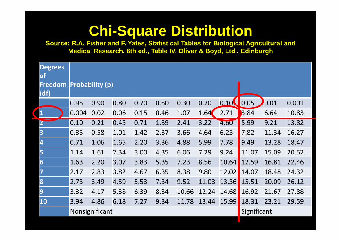
So the Chi-square we calculated =2.668

We need one more thing:The degrees of freedom

• For time being let’s say degrees of freedom are the number of categories we have minus 1

• In this case we have only 2 categories: green and yellow

• So our degrees of freedom are 2 - 1 = 1

Now we want to know, with a confidence level of say 95 %, if the

deviation is just chance. i.e. there is no more than a 5%

possibility that our observations are due to something other than chance .

So we compare our calculated chi-square against the chi-square

distribution

Chi-Square DistributionSource: R.A. Fisher and F. Yates, Statistical Table s for Biological Agricultural and

Medical Research, 6th ed., Table IV, Oliver & Boyd, Ltd., Edinburgh

Degrees

of

Freedom

(df)

Probability (p)

0.95 0.90 0.80 0.70 0.50 0.30 0.20 0.10 0.05 0.01 0.001

1 0.004 0.02 0.06 0.15 0.46 1.07 1.64 2.71 3.84 6.64 10.83

2 0.10 0.21 0.45 0.71 1.39 2.41 3.22 4.60 5.99 9.21 13.82

3 0.35 0.58 1.01 1.42 2.37 3.66 4.64 6.25 7.82 11.34 16.27

4 0.71 1.06 1.65 2.20 3.36 4.88 5.99 7.78 9.49 13.28 18.47

5 1.14 1.61 2.34 3.00 4.35 6.06 7.29 9.24 11.07 15.09 20.52

6 1.63 2.20 3.07 3.83 5.35 7.23 8.56 10.64 12.59 16.81 22.46

7 2.17 2.83 3.82 4.67 6.35 8.38 9.80 12.02 14.07 18.48 24.32

8 2.73 3.49 4.59 5.53 7.34 9.52 11.03 13.36 15.51 20.09 26.12

9 3.32 4.17 5.38 6.39 8.34 10.66 12.24 14.68 16.92 21.67 27.88

10 3.94 4.86 6.18 7.27 9.34 11.78 13.44 15.99 18.31 23.21 29.59

Nonsignificant Significant

Chi-Square DistributionSource: R.A. Fisher and F. Yates, Statistical Table s for Biological Agricultural and

Medical Research, 6th ed., Table IV, Oliver & Boyd, Ltd., Edinburgh

Degrees

of

Freedom

(df)

Probability (p)

0.95 0.90 0.80 0.70 0.50 0.30 0.20 0.10 0.05 0.01 0.001

1 0.004 0.02 0.06 0.15 0.46 1.07 1.64 2.71 3.84 6.64 10.83

2 0.10 0.21 0.45 0.71 1.39 2.41 3.22 4.60 5.99 9.21 13.82

3 0.35 0.58 1.01 1.42 2.37 3.66 4.64 6.25 7.82 11.34 16.27

4 0.71 1.06 1.65 2.20 3.36 4.88 5.99 7.78 9.49 13.28 18.47

5 1.14 1.61 2.34 3.00 4.35 6.06 7.29 9.24 11.07 15.09 20.52

6 1.63 2.20 3.07 3.83 5.35 7.23 8.56 10.64 12.59 16.81 22.46

7 2.17 2.83 3.82 4.67 6.35 8.38 9.80 12.02 14.07 18.48 24.32

8 2.73 3.49 4.59 5.53 7.34 9.52 11.03 13.36 15.51 20.09 26.12

9 3.32 4.17 5.38 6.39 8.34 10.66 12.24 14.68 16.92 21.67 27.88

10 3.94 4.86 6.18 7.27 9.34 11.78 13.44 15.99 18.31 23.21 29.59

Nonsignificant Significant

We find our chi-square value of 2.668 < 2.71SO

The Deviations observed are just chance; and therefore

The findings are compatible with the Mendelian expectations.

And there are many other types of statistical analyses suitable for other

cases, which we will come back to later…

Let’s look at just mapping the data in a graph… what can it tell us?

Cross -sectional And Longitudinal Studies

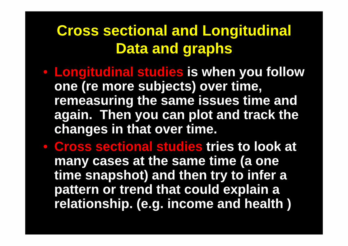
Cross sectional and Longitudinal Data and graphs

• Longitudinal studies is when you follow one (re more subjects) over time, remeasuring the same issues time and again. Then you can plot and track the changes in that over time.

• Cross sectional studies tries to look at many cases at the same time (a one time snapshot) and then try to infer a pattern or trend that could explain a relationship. (e.g. income and health )

Women in parliament and women’s income (cross sectional data)

Economic growth and trust in Government are related

Trust in Government4.5

4

3.5

3

2.5

2

1.5

1

0.5

00-4 -2 2 4 6 8

Growth of per capita GDP (percent per year)

Russia1995

Czech Republic

1995x

x

Implicit assumption: the cases are comparable: i.e. one could move along

the curve plotting the correlation

Florida and its Residents

Old (Mostly Jewish) Retirees in Florida

Young (Mostly Hispanic) Voters in Florida

So:People in Florida are Hispanic

immigrants when they are young and become retired Jewish New Yorkers

when they grow old!Absurd!

Longitudinal studies can help establish causality:

i.e. more than one time measurement for the same

population or group over time.

But despite obvious weaknesses, there is much that can be derived from data

produced by both cross sectional and longitudinal studies

Source: http://learning2grow.org/2011/01/11/the-sin gle-biggest-predictor-of-obesity-is-low-income/

The relation between Obesity and inequality

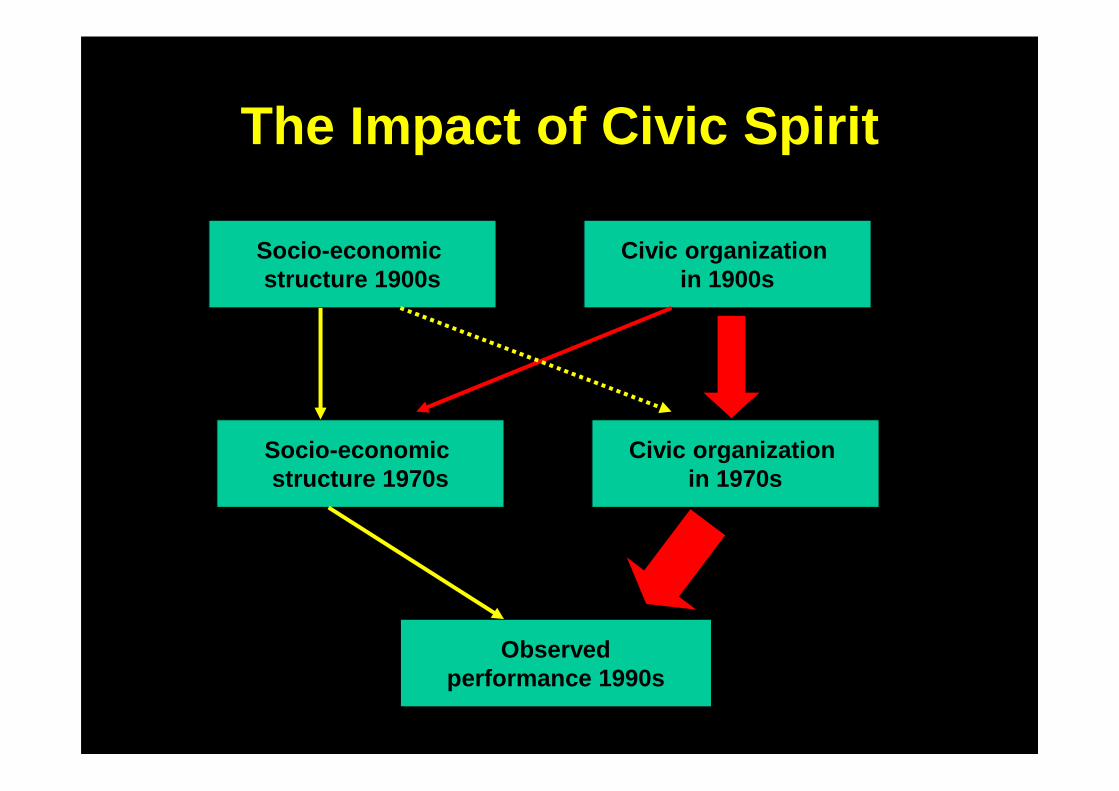
Empirical Evidence: Putnam’s Pioneering Work

Making Democracy Work, Princeton U.P., 1993

The Impact of Civic Spirit

Socio-economic structure 1900s

Observedperformance 1990s

Civic organization in 1900s

Socio-economic structure 1970s

Civic organization in 1970s

So Civic Spirit is the important variable

Civil Society Networks Promote Empowerment

Civil Society forces accountable, responsive and

efficient government…

Is he justified in this conclusion?

What could have invalidated his conclusion?

Correlation and Causality

Correlation ≠ Causation

• Generally, if one factor (A) is observed to be correlated with another factor (B )

• It is sometimes taken for granted that A is causing B, even when no evidence supports it.

• This is a logical fallacy because there are at least five possibilities:

Correlation & Causation:Five Possibilities

• A may be the cause of B.• B may be the cause of A.• Some unknown third factor C may

actually be the cause of both A and B .

A B

• There may be a combination of the above three relationships.

Smoking and Lung Cancer

Smoking and Lung Cancer

• Many studies showed a strong correlation between smoking and increased incidene of Lung cancer

• More detailed studies establishd that heavy smokers increased their probability of lung cancer very significantly.

This is a real case of causality

• Cigarette smoking is the number one risk factor for lung cancer.

• In the United States, cigarette smoking causes about 90% of lung cancers.

• Tobacco smoke is a toxic mix of more than 7,000 chemicals. Many are poisons. At least 70 are known to cause cancer in people or animals.

• People who smoke are 15 to 30 times more likely to get lung cancer or die from lung cancer than people who do not smoke.

• Source: CDC at: http://www.cdc.gov/cancer/lung/basic_info/risk_fact ors.htm

Causality is firmly established

• Even smoking a few cigarettes a day or smoking occasionally increases the risk of lung cancer.

• The more years a person smokes and the more cigarettes smoked each day, the more risk goes up

• References:– Alberg AJ, Ford FG, Samet JM. Epidemiology of lung ca ncer: ACCP evidence-based clinical

practice guidelines (2nd edition). Chest 2007;132(3 Suppl):29S–55S.– U.S. Department of Health and Human Services. The H ealth Consequences of Smoking: A

Report of the Surgeon General (2004).

• Stopping smoking reduces the risk of getting lung cancer

• References: – International Agency for Research on Cancer (IARC). IARC Handbooks of Cancer Prevention

Vol. 11. Tobacco Control: Reversal of Risk after Quitting Smoking. Lyon: International Agency for Research on Cancer (2007).

Additional references:

• International Agency for Research on Cancer (IARC). IARC Monographs on the Evaluation of Carcinogenic Risks to Humans Volume 83: Tobacco Smoke and Involuntary Smoking. Lyon: International Agency for Research on Cancer (2004).

• U.S. Department of Health and Human Services. How Tobacco Smoke Causes Disease: A Report of the Surgeon General (2010).

• U.S. Department of Health and Human Services. The Health Consequences of Smoking: A Report of the Surgeon General (1990).

That was the first possibility: that Correlation does reflect causality…But there are four other possibilities




A B


Firemen Fighting a Fire

Example : B causes A (reverse causation )

• The more firemen fighting a fire, the bigger the fire is observed to be.

• Therefore firemen cause an increase in the size of a fire!

• Actually the opposite: The bigger the fire the more firemen are called in to fight it.




A BC


What does sleeping with your shoes on

produce?

Example 1: Hidden Variable C causes both A & B

• Sleeping with one's shoes on (A) is strongly correlated with waking up with a headache (B).

• Conclusion: sleeping with one's shoes on causes headache [(A) Causes (B)].

• both are caused by a third factor, in this case going to bed drunk, which thereby gives rise to a correlation.

• So the conclusion is false.


• Young children who sleep with the light on are much more likely to develop myopia in later life.

• Therefore , sleeping with the light on causes myopia.

• This is a scientific example that resulted from a study at the University of Pennsylvania Medical Center. Published in the May 13 , 1999 issue of Nature , the study received much coverage at the time in the popular press .

Children sleeping with lights on


• Young children who sleep with the light on are much more likely to develop myopia in later life.

• Therefore , sleeping with the light on causes myopia.

• This is a scientific example that resulted from a study at the University of Pennsylvania Medical Center. Published in the May 13 , 1999 issue of Nature , the study received much coverage at the time in the popular press .


• However, a later study at Ohio State University did not find that infants sleeping with the light on caused the development of myopia.

• It did find a strong link between parental myopia and the development of child myopia, also noting that myopic parents were more likely to leave a light on in their children's bedroom .

• In this case, the cause of both conditions is parental myopia, and the U. of Penn Study conclusion is false.

Drinks, Water and Getting Drunk

Example 3: C causes both A & B(leading many to Spurious conclusions)

• Observation : You get drunk if you drink:– Vodka with water– Whisky with water– Wine with water– Brandy with water

• Hence, since water is only common denominator

• Conclusion : Water makes you drunk• That is a Spurious Conclusion! Because:• Hidden variable : Alcohol in Vodka,

Whisky, Wine and Brandy

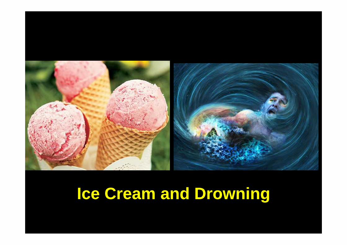
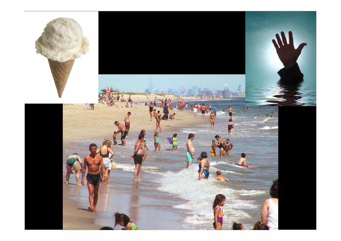
Ice Cream and Drowning

Example 3: Hidden Variable C causes both A & B (variant)

• As ice cream sales increase, the rate of drowning deaths increases sharply.

• Therefore , ice cream consumption causes drowning.

????


• Ice cream is sold during the hot summer months at a much greater rate than during colder times

• It is during these hot summer months that people are more likely to engage in activities involving water, such as swimming.

• The increased drowning deaths are simply caused by more exposure to water-based activities, not ice cream.

• The stated conclusion is false.

Hot Summer Months Increase exposure to both risks o f drowning and increases ice cream consumption




A BC


Carbon Dioxide and Obesity increases


• Since the 1950 s, both the atmospheric CO2 level and obesity levels have increased sharply.

• Hence, atmospheric CO 2 causes obesity.

• Actually, societies have changed, and populations tend to be more sedentary and eat more fatty foods and also consume more energy which, given current technology, raises CO 2 levels.



actually be the cause of both A and B .• There may be a combination of the

above three relationships .• Fifth: It is just a coincidence!

Pirates and Global Warming

Example: Coincidence

• With a decrease in the number of pirates, there has been an increase in global warming over the same period.

• Therefore , global warming is caused by a lack of pirates !

Global Warming has well understood causes and effects

Bottled water and murder

Correlation without causation

• Two observed events are not necessarily related.

For Example: • people drink more bottled water than

they did in the past. There are also more murders than there were in the past.

BUT• we cannot say that drinking bottled

water leads to murder

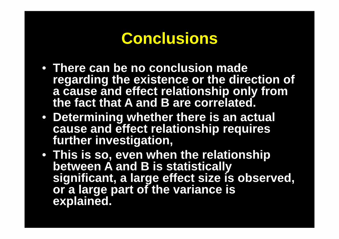
Conclusions

• There can be no conclusion made regarding the existence or the direction of a cause and effect relationship only from the fact that A and B are correlated.

• Determining whether there is an actual cause and effect relationship requires further investigation,

• This is so, even when the relationship between A and B is statistically significant, a large effect size is observed, or a large part of the variance is explained.

Correlation does not imply Causality.

Are two successive measurements enough to establish causality?

Education Studies

Interpreting Causality:The facts

Cold Teacher, Unresponsive Student

Warm Teacher, Responsive Student

Conclusion:Warmer teachers illicit more response from the students

But, Wait…What about…

Teachers are warmer towards more responsive students

Warm Teacher + Responsive Student

Interpreting Causality:The facts

Interpreting Causality:Possible Explanations

Unresponsive Student >> Cold Teacher?

Cold Teacher >> Unresponsive Student ?

Experimental DesignIs how we try to answer these

questions and control for other issues

(That will come later)

Student behavior and Teacher behavior

We will discuss this Later!

Experimental

Design

Correlation

Correlation = Causation

• Correlation: is observing multiple events at the same time

• Causation: is one event leading to another.

• They are not the same.

/

High Voltage Transmission lines and disease

Correlation without causation

• Two observed events are not necessarily related.

For Example: • People who live under high voltage electric

wires tend to have more diseases … hence:

• High voltage wires cause you to be sickNO…

• No, poorer people tend to be the ones who live under high voltage wires, and generally, people who are poorer tend to have more diseases,

Causation

• On the other hand, causation is a one -way direction, one is dependent and the other one is independent. – A only goes to B. – B cannot go to A. – Therefore, the occurrence of B depends on A. – A is a predictor to B.

• Every causation always has got a strong correlation, but not all strong correlation is a causation.

Causation -- Examples

• Anxiety and heart rate in adults . You can say, the higher the anxiety, the more rapid the heart rate or anxiety causes increasing in heart rate. You cannot say that increasing in heart rate causes anxiety.

• Human population and pollution in a given area . The more people in a given area, the greater the pollution. It doesn't mean that the greater the pollution, the more people in that area.

1. Not being what it purports to be; false or fake: " spurious claims ".

2. Apparently but not actually valid: "this spurious reasoning results in nonsense ".

Spurious

Furthermore…

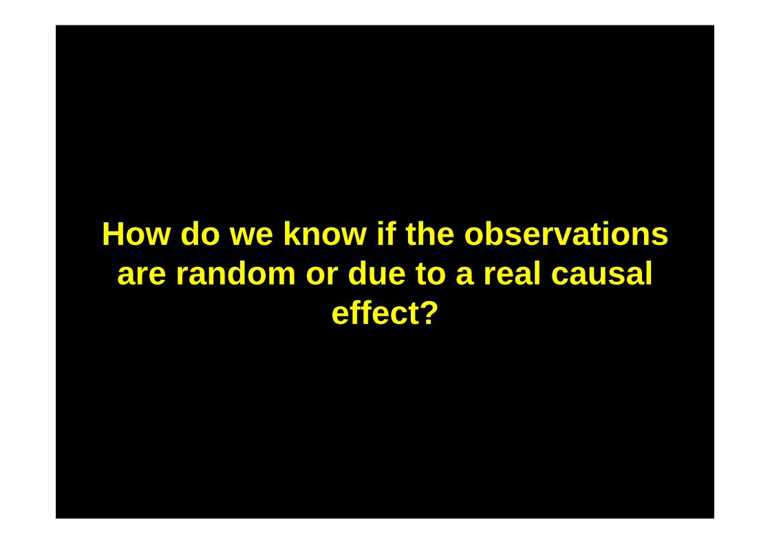
How do we know if the observations are random or due to a real causal

effect?

ANOVAAnalysis Of Variance

• A statistical analysis tool that separates the total variability found within a data set into two components: random and systematic factors.

• The random factors do not have any statistical influence on the given data set, while the systematic factors do.

ANOVAanalysis of variance

• The ANOVA test is used to determine the impact independent variables have on the dependent variable in a regression analysis.

Using cross -sectional data comparisons

While generally true, looking just at these two variables (Malnutrition and Income) hides the complexity of the underlying

relationship.

The Nutrition -Income Relationship

Interventions at different parts of that diagram can affect the outcome

Policy Based On Simple Mapping of

Observations of Different Countries

Education is important for growth, Therefore:

more education = more growth

Coef=0.264058, se=.7839797, t=.34 Other countries

Added -variable Plots of Growth and Education(Quantity)

Conditional years of education

-4

IRN

JOR

ZWE

PHL

JPNROM

ISRAUT

INDCHN NZL

URYGHACOL

NLDTUREGY

ISLITACHE

PRT

TUNMAR

SGP

CYP

NORIRLCHL

KOR

DNK

THAIDN

TWNHKG

ZAFUSABRA

PER

GRCGBRAUSESPMEX

SWEBEL

CAN

●●●●

●

-2 0 2 4

-20

21

-1Con

ditio

nal g

row

th

●

Source: World Bank Policy Research Working Paper 41 22, February 2007. “ The Role of Education Quality in Economic Growth”, Figure 4.2 (b).

Added -variable Plots of Growth and Education (Quality)

Con

ditio

nal g

row

th

Conditional test score

Coef=1.9804387, se=.21707105, t=9.12-1.5 -1 -0.5 0 0.5 1

JOR

BRANOR

CHN

HKG

USA

●●

●●

KOR

TWN

SGP

TUNCYPMYS

FRAFINIRN

IND

ROM

●●

●●●●●

●●

●●●●●

●

●●

IDNMAR

●●●

GHAPHLPER

ZAFARGCHN

ZWE

● ●

● Other countries

-40

2-2

4

Source: World Bank Policy Research Working Paper 41 22, February 2007. “ The Role of Education Quality in Economic Growth” Figure 4.2 (a): .

Must focus on Educational Quality not just Quantity

Furthermore, educational inequality is correlated with income inequality

Inequality of Educational Quality and Earnings

Source: Nickell (2004) Figure 2.4.

3.0

2.5

2.0

1.5

3.5

4.0

3.0

DEN

NORSWE

GER

NET

FINBEL

SWI

AUS

IREUK

CANUSA

1.3 1.5 1.7 1.9

Test score inequality

Ear

ning

s in

equa

lity

Note: Measure of inequality is the ratio of ninth d ecile to first decile in both cases; test performan ce refers to prose literacy in the International Adult Litera cy Survey.

These very simple graphs help give insights for policy

Policy Based On Simple Mapping of Observations Over

Time

We will not discuss here Tipping Points

(leave that to another discussion)

Sustainable development does not mean that people

will live worse…

Let’s look at income and health

Life Expectancy versus Per Capita GNP Best Fit Relation by Decade

(Thousands)

Per Capita GNP (1980 US$)

Life

Exp

ecta

ncy

19871980

1970

19501961

20

30

40

50

60

70

80

0 2 4 6 8 10 12 14 16 18 20

Life Expectancy versus Per Capita GNP Best Fit Relation by Decade

(Thousands)

Per Capita GNP (1980 US$)

Life

Exp

ecta

ncy

19871980

1970

19501961

20

30

40

50

60

70

80

0 2 4 6 8 10 12 14 16 18 20

Policy Counts!

So, even limited data points can tell us very important things

about key issues

So… Let’s Check Again..

Are we sinking? Or Swimming?

Is everyone swimming?

Some may be already flying…

Thank You

Lecture -- 3 -- Start - University of Pittsburghsuper7/51011-52001/51381.pdf · Lecture # 3:...

Documents

Transcript of Lecture -- 3 -- Start - University of Pittsburghsuper7/51011-52001/51381.pdf · Lecture # 3:...