Lecture 3Protein binding networks

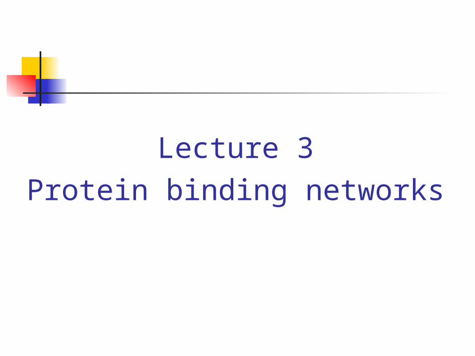
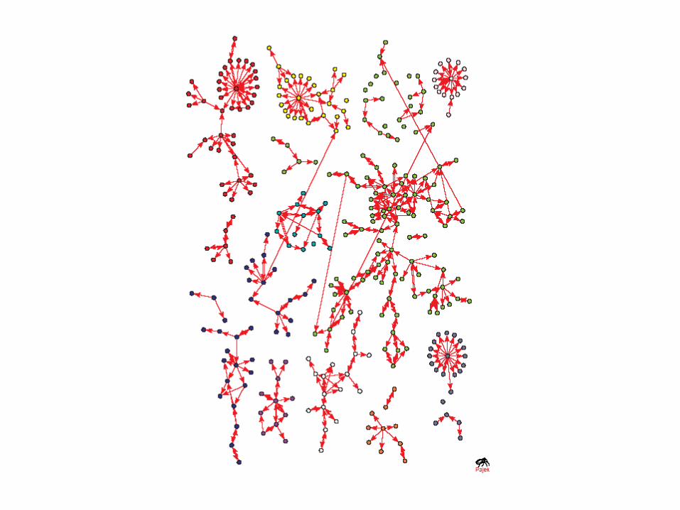
C. elegans PPI from Li et al. (Vidal’s lab), Science (2004)

Genome-wide protein binding networks

Nodes - proteins Edges - protein-

protein binding interactions

Functions Structural (keratin) Functional (ribosome) regulation/signaling

(kinases) etc

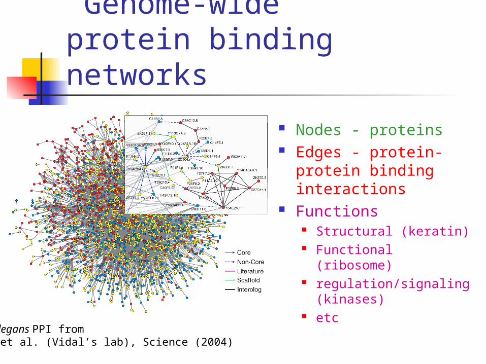
How much data is out there?

Species Set nodes edges # of sources

S.cerevisiae HTP-PI 4,500 13,000 5

LC-PI 3,100 20,000 3,100

D.melanogaster HTP-PI 6,800 22,000 2

C.elegans HTP-PI 2,800 4,500 1

H.sapiens LC-PI 6,400 31,000 12,000

HTP-PI 1,800 3,500 2 H. pylori HTP-PI 700 1,500 1

P. falciparum HTP-PI 1,300 2,800 1

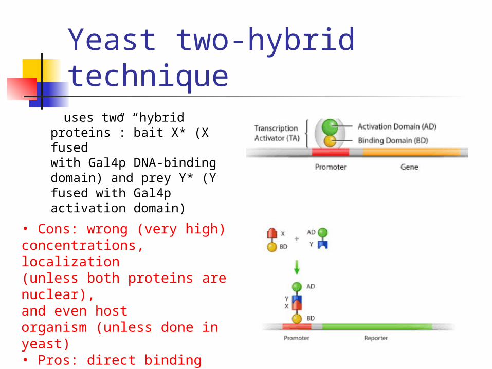
Yeast two-hybrid technique

uses two “hybrid proteins”: bait X* (X fused

with Gal4p DNA-binding domain) and prey Y* (Y fused with Gal4p activation domain)

• Cons: wrong (very high) concentrations, localization (unless both proteins are nuclear), and even host organism (unless done in yeast) • Pros: direct binding events• Main source of noise: self-activating baits

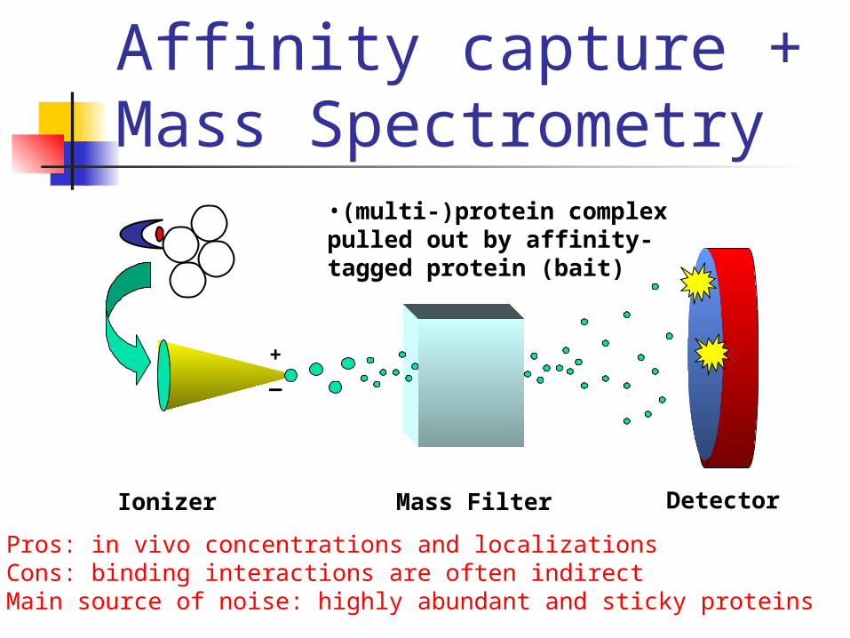
Affinity capture +Mass Spectrometry

Ionizer

•(multi-)protein complex pulled out by affinity-tagged protein (bait)

+_

Mass Filter Detector

• Pros: in vivo concentrations and localizations• Cons: binding interactions are often indirect• Main source of noise: highly abundant and sticky proteins

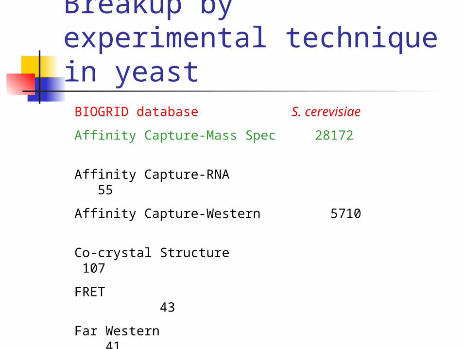
Breakup by experimental technique in yeast

BIOGRID database S. cerevisiae

Affinity Capture-Mass Spec 28172

Affinity Capture-RNA 55

Affinity Capture-Western 5710

Co-crystal Structure 107

FRET 43

Far Western 41

Two-hybrid 11935

Total 46063

What are the common topological features?

1. Broad distribution of the number of interaction partners of individual proteins

• What’s behind this broad distribution?

• Three explanations were proposed:

• EVOLUTIONARY (duplication-divergence models)• BIOPHYSICAL (stickiness due to surface hydrophobicity)• FUNCTIONAL(tasks of vastly different complexity)

From YY. Shi, GA. Miller., H. Qian., and K. Bomsztyk, PNAS 103, 11527 (2006)

Evolutionary explanation:duplication-divergence models A. Vazquez, A. Flammini, A. Maritan, and A. Vespignani. Modelling

of protein interaction networks. cond-mat/0108043, (2001) published in ComPlexUs 1, 38 (2003)

Followed by R. V. Sole, R. Pastor-Satorras, E. Smith, T. B. Kepler, A model of large-scale proteome evolution, cond-mat/0207311 (2002) published in Advances in Complex Systems 5, 43 (2002)

Then many others including I.Ispolatov, I., Krapivsky, P.L., Yuryev, A., Duplication-divergence model of protein interaction network, Physical Review, E 71, 061911, 2005.

• Network has to grow• Preferential attachment in disguise: as ki grows so is the probability to duplicate one of the neighbors

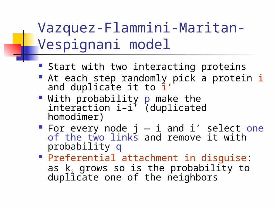
Vazquez-Flammini-Maritan-Vespignani model Start with two interacting proteins At each step randomly pick a protein i

and duplicate it to i’ With probability p make the interaction

i–i’ (duplicated homodimer) For every node j — i and i’ select one of

the two links and remove it with probability q

Preferential attachment in disguise: as ki grows so is the probability to duplicate one of the neighbors

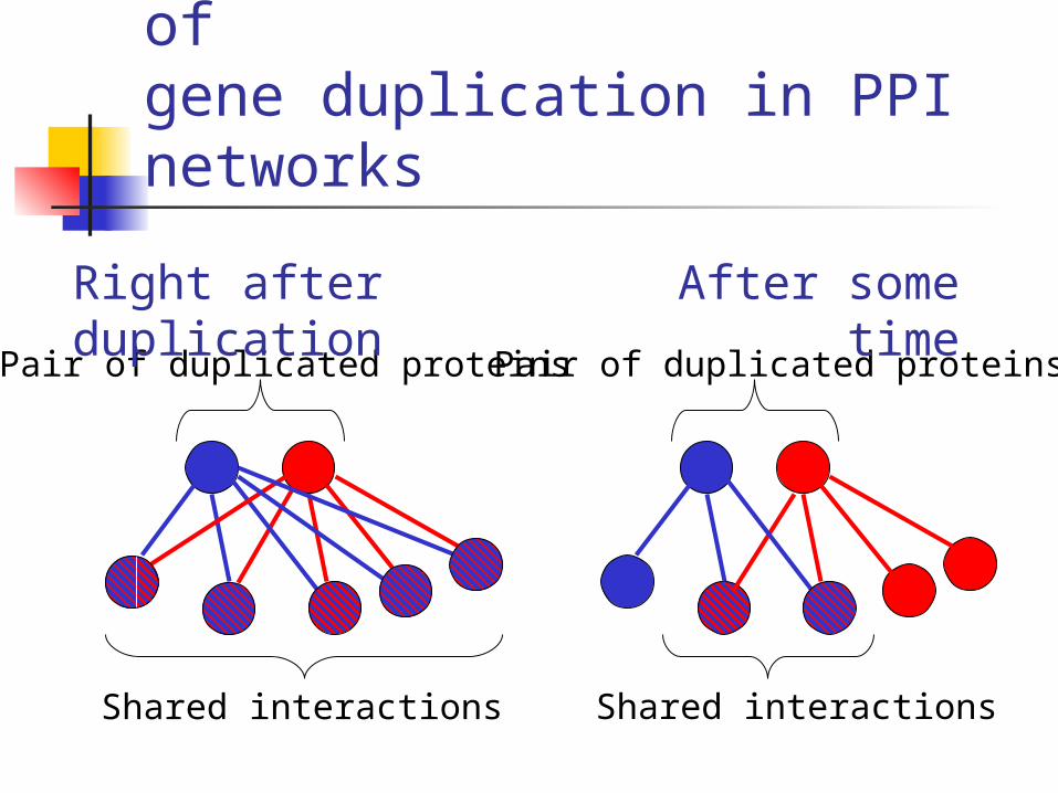
Tell-tale signs of gene duplication in PPI networks

Pair of duplicated proteins

Shared interactions

Pair of duplicated proteins

Shared interactions

Right after duplication

After some time

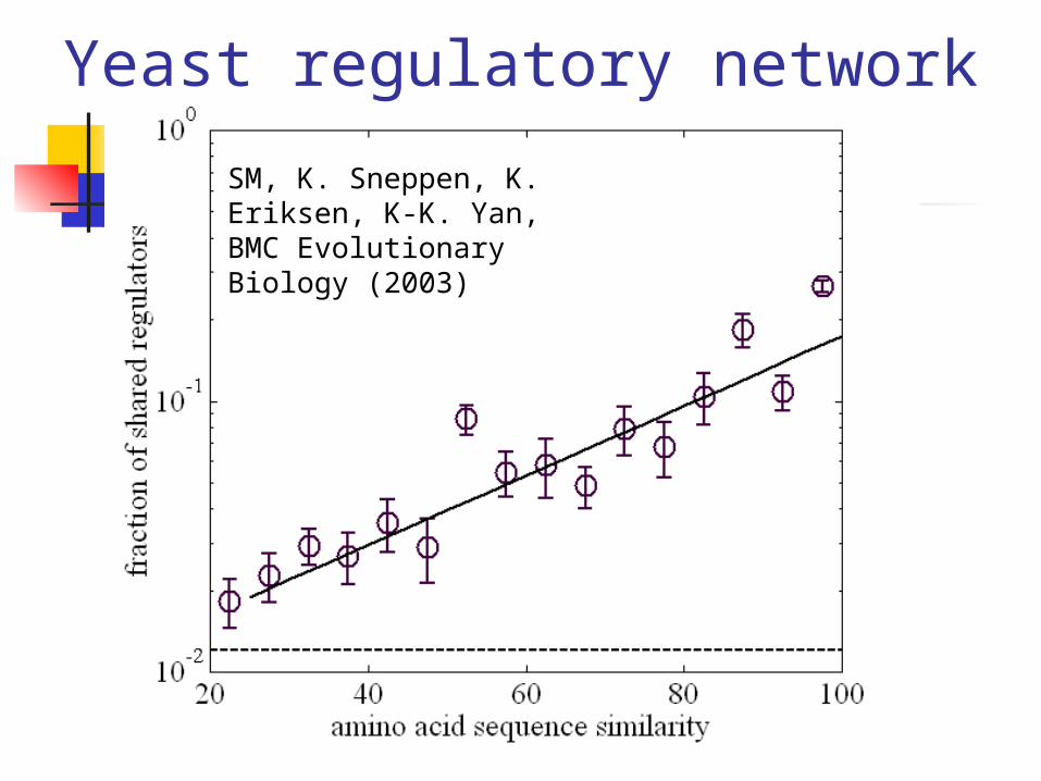
Yeast regulatory network

SM, K. Sneppen, K. Eriksen, K-K. Yan, BMC Evolutionary Biology (2003)

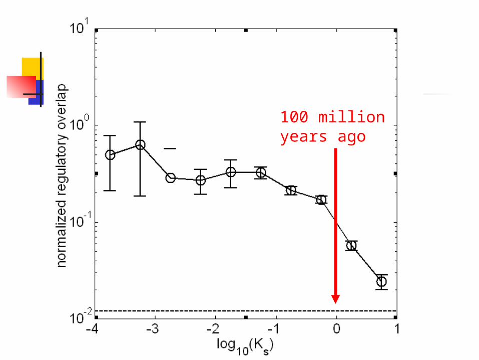
100 million years ago

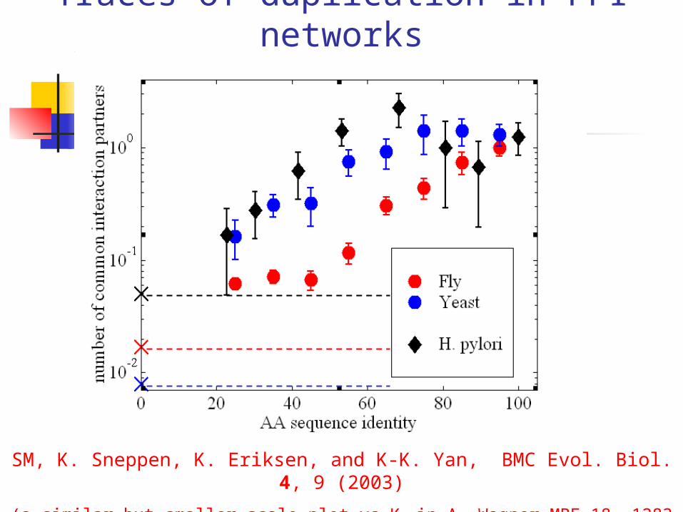
Traces of duplication in PPI networks

SM, K. Sneppen, K. Eriksen, and K-K. Yan, BMC Evol. Biol. 4, 9 (2003)

(a similar but smaller scale-plot vs Ks in A. Wagner MBE 18, 1283 (2001)

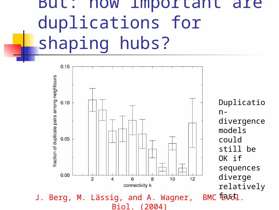
But: how important are duplications for shaping hubs?

J. Berg, M. Lässig, and A. Wagner, BMC Evol. Biol. (2004)

Duplication-divergence models could still be OK if sequences diverge relatively fast

Biophysical explanation:“stickiness” models G. Caldarelli, A. Capocci, P. De Los Rios, M.A. Munoz, Scale-free

Networks without Growth or Preferential Attachment: Good get Richer, cond-mat/0207366, (2002) published in PRL (2002)

Followed by Deeds, E.J. and Ashenberg, O. and Shakhnovich, E.I., A simple physical model for scaling in protein-protein interaction networks, PNAS (2006)

Then others including Yi Y. Shi, G.A. Miller, H. Qian, and K. Bomsztyk, Free-energy distribution of binary protein–protein binding suggests cross-species interactome differences, PNAS (2006).

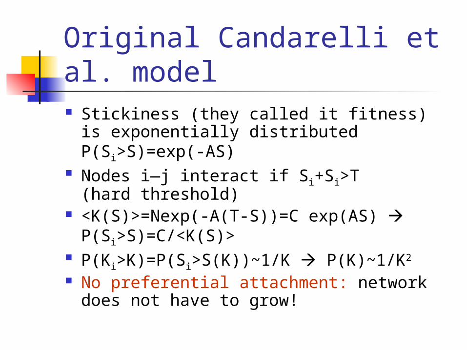
Original Candarelli et al. model Stickiness (they called it fitness) is

exponentially distributed P(Si>S)=exp(-AS) Nodes i—j interact if Si+Si>T

(hard threshold) <K(S)>=Nexp(-A(T-S))=C exp(AS)

P(Si>S)=C/<K(S)> P(Ki>K)=P(Si>S(K))~1/K P(K)~1/K2

No preferential attachment: network does not have to grow!

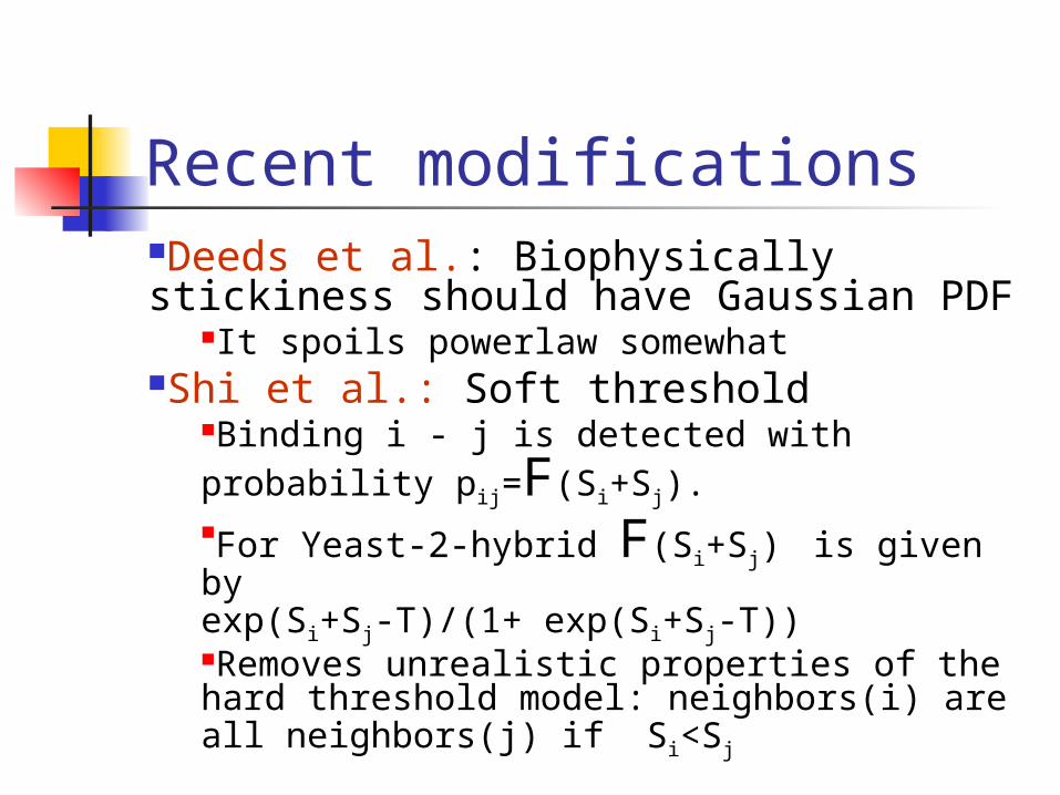
Recent modificationsDeeds et al.: Biophysically stickiness should have Gaussian PDF

It spoils powerlaw somewhatShi et al.: Soft threshold

Binding i - j is detected with probability pij=F(Si+Sj). For Yeast-2-hybrid F(Si+Sj) is given by exp(Si+Sj-T)/(1+ exp(Si+Sj-T))Removes unrealistic properties of the hard threshold model: neighbors(i) are all neighbors(j) if Si<Sj

There are just TOO MANY homodimers

• Null-model: Pself ~<k>/NN (r)

dimer =N Pself

= <k>• Not surprising ashomodimers have many functional roles

I. Ispolatov, A. Yuryev, I. Mazo, and SM, 33, 3629 NAR (2005)

N (r)dimer

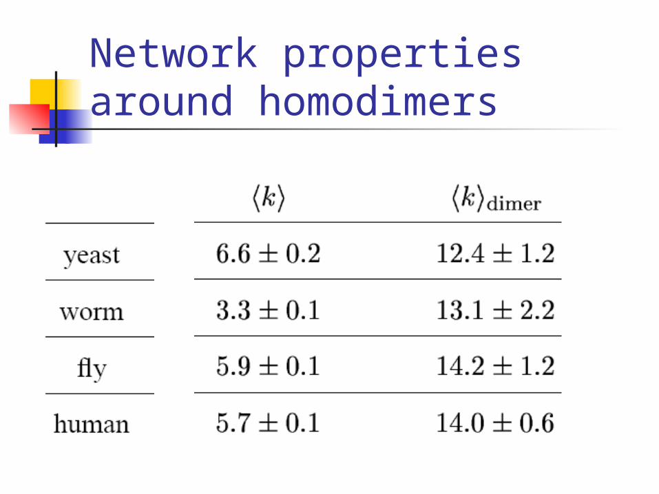
Network properties around homodimers

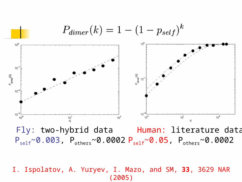
Human: literature dataPself~0.05, Pothers~0.0002

Fly: two-hybrid dataPself~0.003, Pothers~0.0002

I. Ispolatov, A. Yuryev, I. Mazo, and SM, 33, 3629 NAR (2005)

Our interpretation Both the number of interaction partners Ki and the

likelihood to self-interact are proportional to the same “stickiness” of the protein Si which could depend on

the number of hydrophobic residues on the surface protein abundance its’ popularity (in networks taken from many small-scale

experiments) etc.

In random networks pdimer(K)~K2 not ~K like we observe empirically

I. Ispolatov, A. Yuryev, I. Mazo, and SM, 33, 3629 NAR (2005)

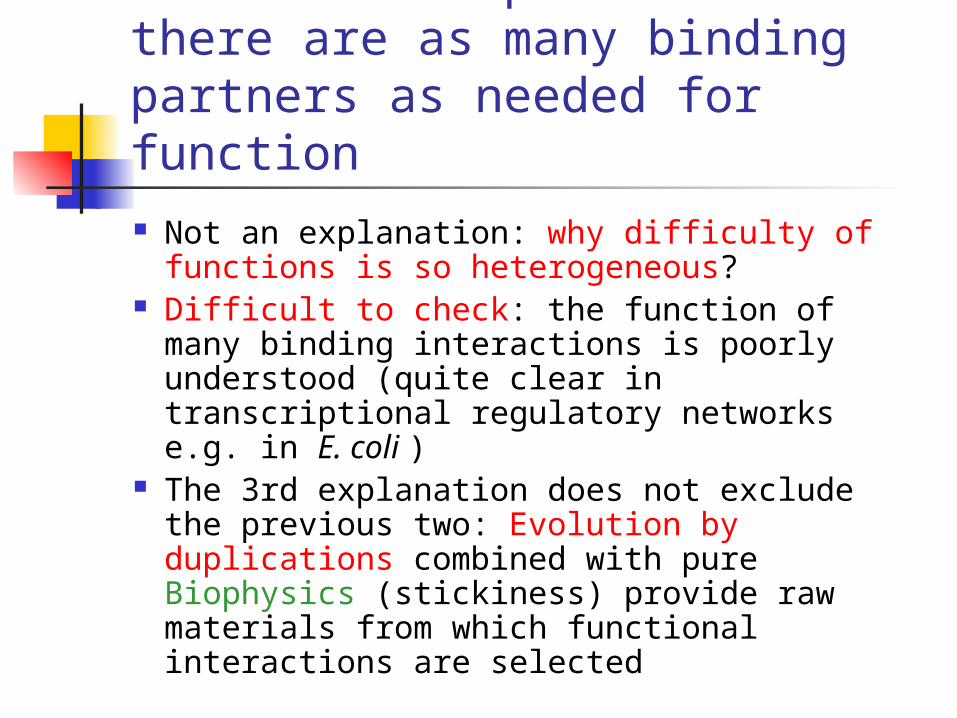
Functional explanation:there are as many binding partners as needed for function Not an explanation: why difficulty of

functions is so heterogeneous? Difficult to check: the function of many

binding interactions is poorly understood (quite clear in transcriptional regulatory networks e.g. in E. coli )

The 3rd explanation does not exclude the previous two: Evolution by duplications combined with pure Biophysics (stickiness) provide raw materials from which functional interactions are selected

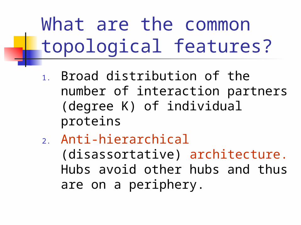
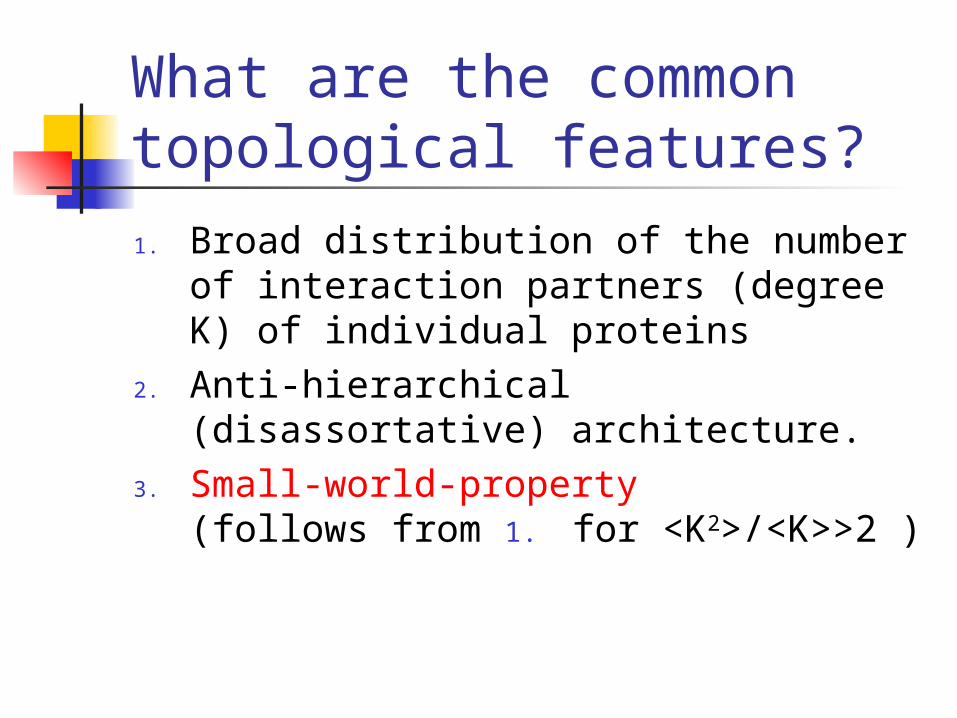
What are the common topological features?

1. Broad distribution of the number of interaction partners (degree K) of individual proteins

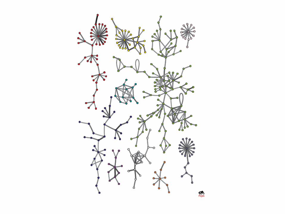
2. Anti-hierarchical (disassortative) architecture. Hubs avoid other hubs and thus are on a periphery.

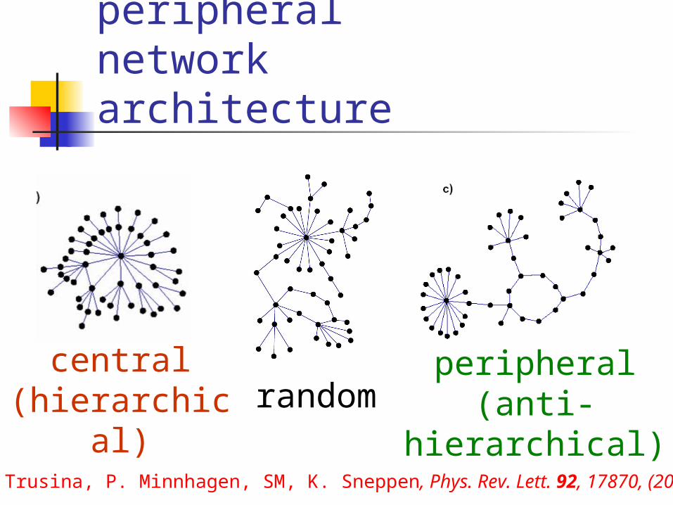
Central vs peripheral network architecture

central(hierarchical)

peripheral(anti-

hierarchical)A. Trusina, P. Minnhagen, SM, K. Sneppen, Phys. Rev. Lett. 92, 17870, (2004)

random

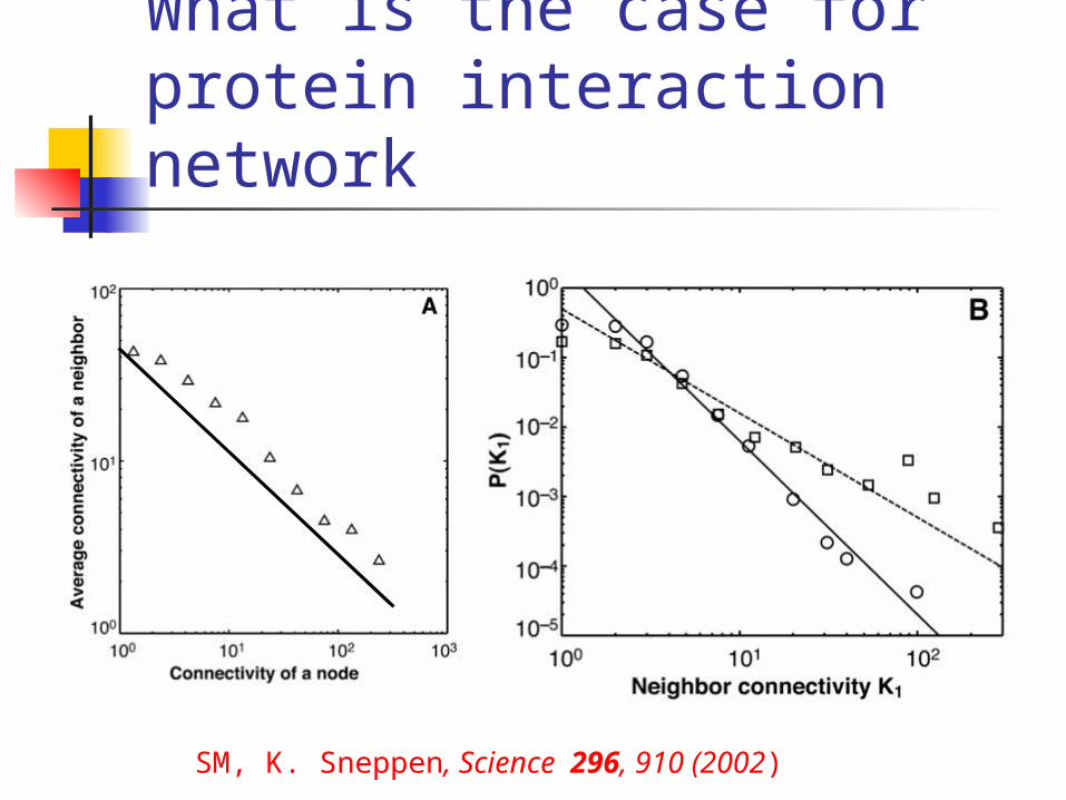
What is the case for protein interaction network

SM, K. Sneppen, Science 296, 910 (2002)

What are the common topological features?

1. Broad distribution of the number of interaction partners (degree K) of individual proteins

2. Anti-hierarchical (disassortative) architecture.

3. Small-world-property (follows from 1. for <K2>/<K>>2 )

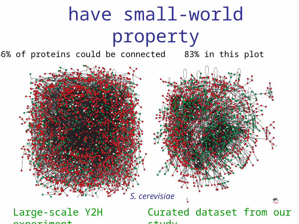
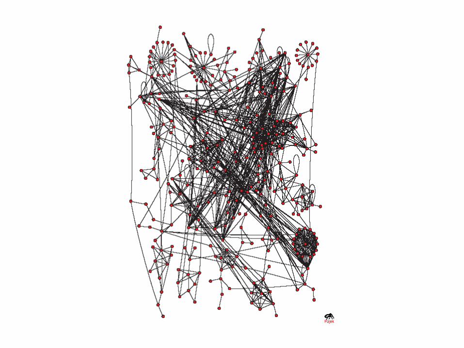
Protein binding networkshave small-world property

Curated dataset from our study

83% in this plot

Large-scale Y2H experiment

S. cerevisiae

86% of proteins could be connected

Why small-world matters? Claims of “robustness” of this network

architecture come from studies of the Internet where breaking up the network is a disaster

For PPI networks it is the OPPOSITE: interconnected networks present a problem

In a small-world network equilibrium concentrations of all proteins are coupled to each other

Danger of undesirable cross-talk

Going beyond topology and modeling the equilibrium and

kinetics

SM, K. Sneppen, I. Ispolatov, q-bio/0611026; SM, I. Ispolatov, PNAS in press (2007)

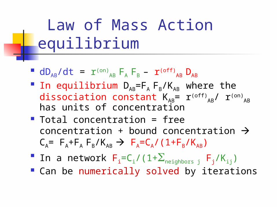
Law of Mass Action equilibrium

dDAB/dt = r(on)AB FA FB – r(off)

AB DAB

In equilibrium DAB=FA FB/KAB where the dissociation constant KAB= r(off)

AB/ r(on)AB

has units of concentration Total concentration = free concentration

+ bound concentration CA= FA+FA

FB/KAB FA=CA/(1+FB/KAB) In a network Fi=Ci/(1+neighbors j Fj/Kij) Can be numerically solved by iterations

What is needed to model? A reliable network of reversible (non-catalytic)

protein-protein binding interactions CHECK! e.g. physical interactions between yeast

proteins in the BIOGRID database with 2 or more citations. Most are reversible: e.g. only 5% involve a kinase

Total concentrations Ci and sub-cellular localizations of all proteins CHECK! genome-wide data for yeast in 3 Nature papers

(2003, 2003, 2006) by the group of J. Weissman @ UCSF. VERY BROAD distribution: Ci ranges between 50 and 106

molecules/cell Left us with 1700 yeast proteins and ~5000 interactions

in vivo dissociation constants Kij OOPS! . High throughput experimental techniques are

not there yet

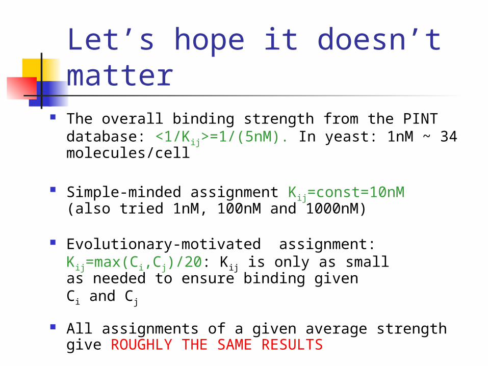
Let’s hope it doesn’t matter

The overall binding strength from the PINT database: <1/Kij>=1/(5nM). In yeast: 1nM ~ 34 molecules/cell

Simple-minded assignment Kij=const=10nM(also tried 1nM, 100nM and 1000nM)

Evolutionary-motivated assignment:Kij=max(Ci,Cj)/20: Kij is only as small as needed to ensure binding given Ci and Cj

All assignments of a given average strength give ROUGHLY THE SAME RESULTS

Robustness with respect to assignment of Kij

Spearman rank correlation: 0.89

Pearson linear correlation: 0.98

Bound concentrations: Dij

Spearman rank correlation: 0.89

Pearson linear correlation: 0.997

Free concentrations: Fi

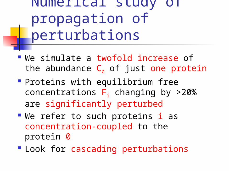
Numerical study of propagation of perturbations

We simulate a twofold increase of the abundance C0 of just one protein

Proteins with equilibrium free concentrations Fi changing by >20% are significantly perturbed

We refer to such proteins i as concentration-coupled to the protein 0

Look for cascading perturbations

Resistor network analogy Conductivities ij – dimer (bound)

concentrations Dij

Losses to the ground iG – free (unbound)

concentrations Fi

Electric potentials – relative changes in free concentrations (-1)L Fi/Fi

Injected current – initial perturbation C0

SM, K. Sneppen, I. Ispolatov, arxiv.org/abs/q-bio.MN/0611026;

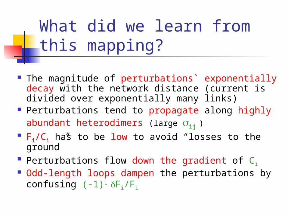
What did we learn from this mapping?

The magnitude of perturbations` exponentially decay with the network distance (current is divided over exponentially many links)

Perturbations tend to propagate along highly abundant heterodimers (large ij )

Fi/Ci has to be low to avoid “losses to the ground”

Perturbations flow down the gradient of Ci

Odd-length loops dampen the perturbations by confusing (-1)L Fi/Fi

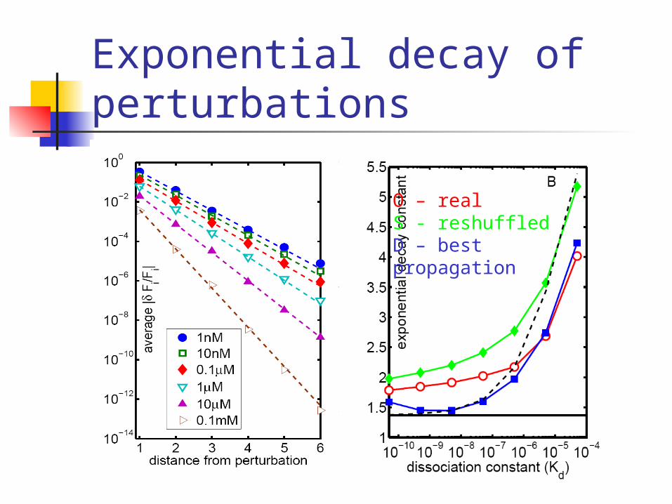
Exponential decay of perturbations

O – realS - reshuffledD – best propagation

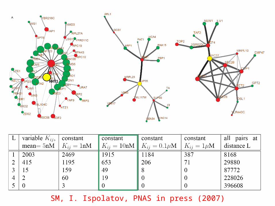
SM, I. Ispolatov, PNAS in press (2007)

HHT1

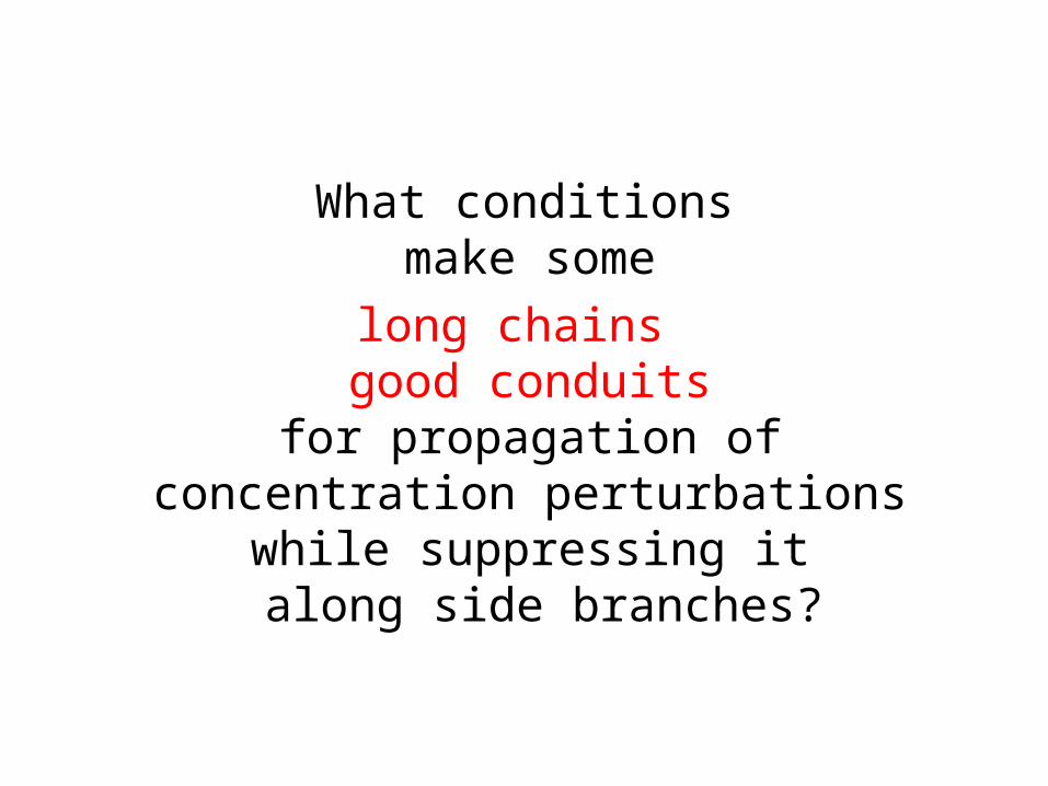
What conditionsmake some

long chains good conduits

for propagation of concentration perturbations

while suppressing it along side branches?

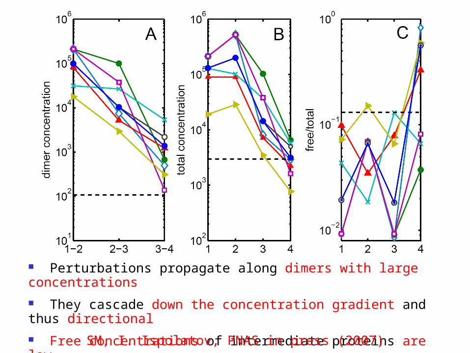
Perturbations propagate along dimers with large concentrations

They cascade down the concentration gradient and thus directional

Free concentrations of intermediate proteins are lowSM, I. Ispolatov, PNAS in press (2007)

Implications of our results

Cross-talk via small-world topology is suppressed, but… Good news: on average perturbations via

reversible binding rapidly decay Still, the absolute number of

concentration-coupled proteins is large In response to external stimuli levels of

several proteins could be shifted. Cascading changes from these perturbations could either cancel or magnify each other.

Our results could be used to extend the list of perturbed proteins measured e.g. in microarray experiments

Genetic interactions Propagation of concentration

perturbations is behind many genetic interactions e.g. of the “dosage rescue” type

We found putative “rescued” proteins for 136 out of 772 such pairs (18% of the total, P-value 10-

216)

SM, I. Ispolatov, PNAS in press (2007)

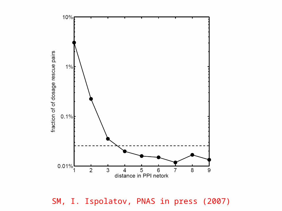
SM, I. Ispolatov, PNAS in press (2007)

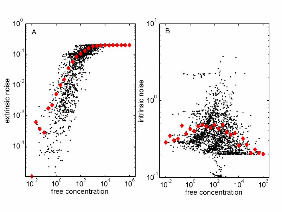
Intra-cellular noise Noise is measured for total concentrations

Ci (Newman et al. Nature (2006)) Needs to be converted in biologically

relevant bound (Dij) or free (Fi) concentrations

Different results for intrinsic and extrinsic noise

Intrinsic noise could be amplified (sometimes as much as 30 times!)

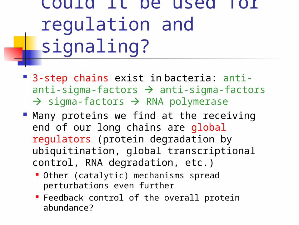
Could it be used for regulation and signaling?

3-step chains exist in bacteria: anti-anti-sigma-factors anti-sigma-factors sigma-factors RNA polymerase

Many proteins we find at the receiving end of our long chains are global regulators (protein degradation by ubiquitination, global transcriptional control, RNA degradation, etc.) Other (catalytic) mechanisms spread perturbations

even further Feedback control of the overall protein

abundance?

NOW BACK TO TOPOLOGY

Summary There are many kinds of protein networks Networks in more complex organisms are more

interconnected Most have hubs – highly connected proteins and

a broad (~scale-free) distribution of degrees Hubs often avoid each other (networks are anti-

hierarchical or disassortative) Networks evolve by gene duplications There are many self-interacting proteins.

Likelihood to self-interact and the degree K both scale with protein’s “stickiness”

THE END

Why so many genes could be deleted without any

consequences?

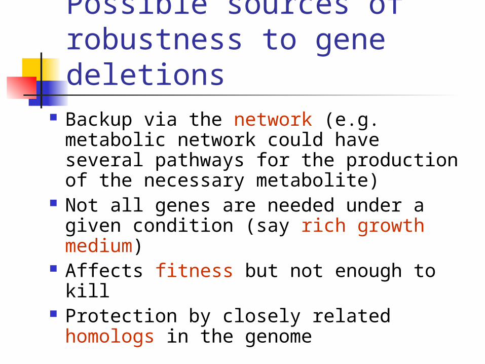
Possible sources of robustness to gene deletions

Backup via the network (e.g. metabolic network could have several pathways for the production of the necessary metabolite)

Not all genes are needed under a given condition (say rich growth medium)

Affects fitness but not enough to kill Protection by closely related

homologs in the genome

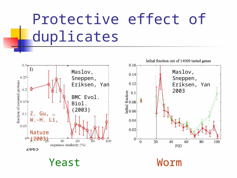
Protective effect of duplicates

Gu, et al 2003Maslov, Sneppen,

Eriksen, Yan 2003

Yeast Worm

Maslov, Sneppen, Eriksen, Yan 2003

Z. Gu, … W.-H. Li, Nature (2003)

Maslov, Sneppen, Eriksen, Yan BMC Evol. Biol.(2003)