Lecture 3 Outline: Tues, Jan 20

• Chapter 1.3

• Probability model for 2-group randomized experiment.

• Hypothesis testing review

• Randomization test p-value

• Principle of control in experimental design

Vocabulary of Experiments

• A study is an experiment when we actually do something to people, animals or objects to observe the response.

• Experimental units are the things to which treatments are applied, e.g., people, rats, samples of materials or pieces of land.

• When units are human beings, they are called subjects.• A specific experimental condition applied to the units is

called a treatment. • The “control” refers to a treatment that is considered a

baseline for comparing all other treatments.• Creativity study: Experimental units? Treatments?

Probability Model for 2-treatment Randomized

Experiment• Creativity Study

– Chance mechanism for randomizing units to treatment groups ensures that every subset of 24 subjects gets the same chance of becoming intrinsic group

– For example, 23 red and 24 black cards could be shuffled and dealt, one to each subject and the subjects with black cards would be the intrinsic group.

– Tables of random numbers can be used to assign units to groups (assign the units with the 24 highest numbers to group 1).

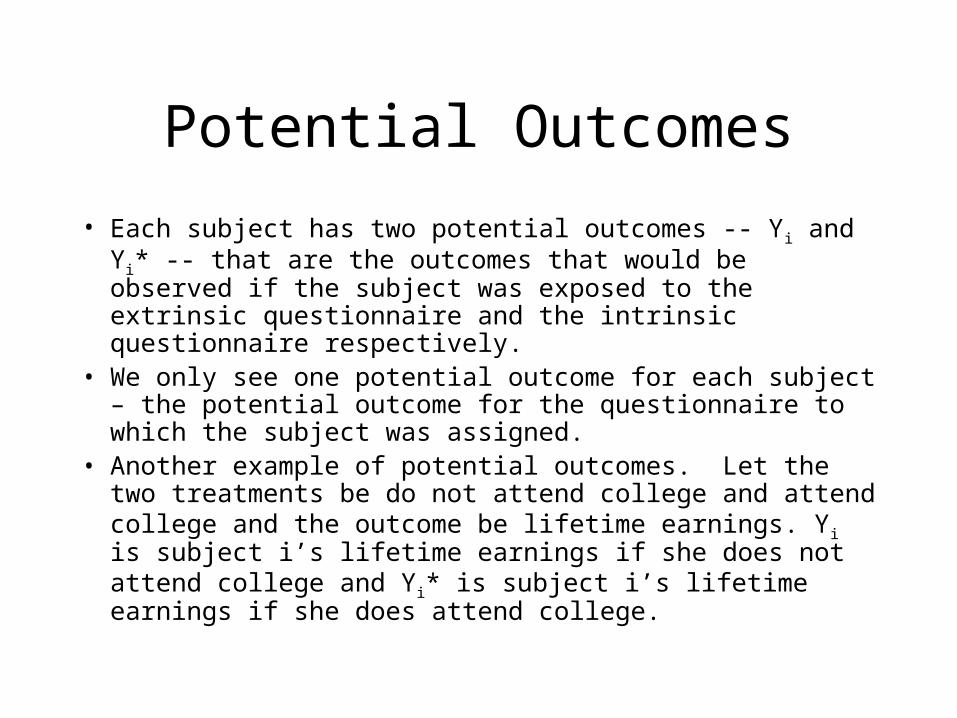
Potential Outcomes

• Each subject has two potential outcomes -- Yi and Yi* -- that are the outcomes that would be observed if the subject was exposed to the extrinsic questionnaire and the intrinsic questionnaire respectively.

• We only see one potential outcome for each subject – the potential outcome for the questionnaire to which the subject was assigned.

• Another example of potential outcomes. Let the two treatments be do not attend college and attend college and the outcome be lifetime earnings. Yi is subject i’s lifetime earnings if she does not attend college and Yi* is subject i’s lifetime earnings if she does attend college.

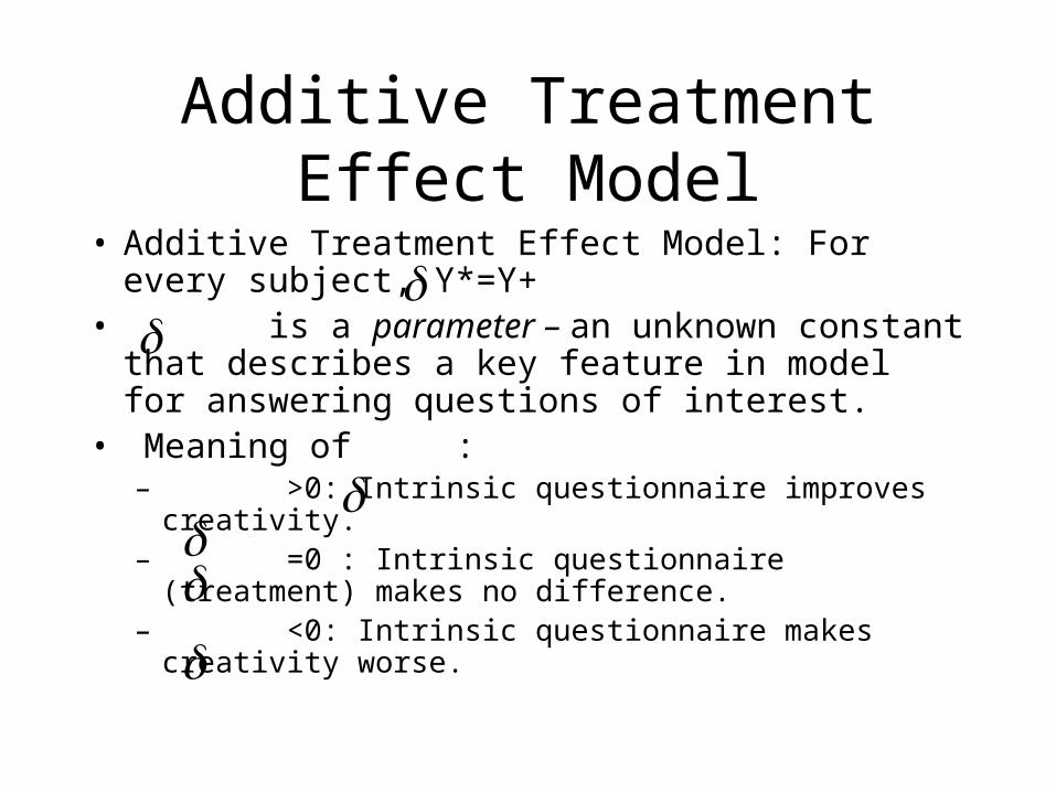
Additive Treatment Effect Model

• Additive Treatment Effect Model: For every subject, Y*=Y+

• is a parameter – an unknown constant that describes a key feature in model for answering questions of interest.

• Meaning of :– >0: Intrinsic questionnaire improves creativity.– =0 : Intrinsic questionnaire (treatment) makes no

difference.– <0: Intrinsic questionnaire makes creativity worse.

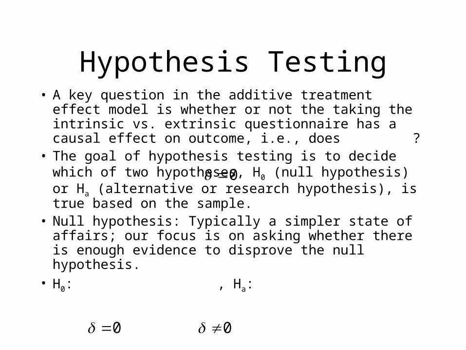
Hypothesis Testing• A key question in the additive treatment effect model is

whether or not the taking the intrinsic vs. extrinsic questionnaire has a causal effect on outcome, i.e., does ?

• The goal of hypothesis testing is to decide which of two hypotheses, H0 (null hypothesis) or Ha (alternative or research hypothesis), is true based on the sample.

• Null hypothesis: Typically a simpler state of affairs; our focus is on asking whether there is enough evidence to disprove the null hypothesis.

• H0: , Ha:

0

0

0

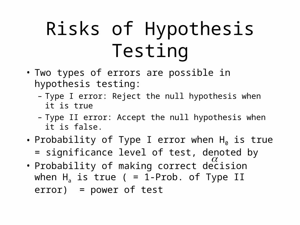
Risks of Hypothesis Testing

• Two types of errors are possible in hypothesis testing:– Type I error: Reject the null hypothesis when it is true

– Type II error: Accept the null hypothesis when it is false.

• Probability of Type I error when H0 is true = significance level of test, denoted by

• Probability of making correct decision when Ha is true ( = 1-Prob. of Type II error) = power of test

Hypothesis Testing in the Courtroom

• Null hypothesis: The defendant is innocent• Alternative hypothesis: The defendant is guilty• The goal of the procedure is to determine whether

there is enough evidence to conclude that the alternative hypothesis is true. The burden of proof is on the alternative hypothesis.

• Two types of errors:– Type I error: Reject null hypothesis when null hypothesis is

true (convict an innocent defendant)– Type II error: Do not reject null hypothesis when null is

false (fail to convict a guilty defendant)

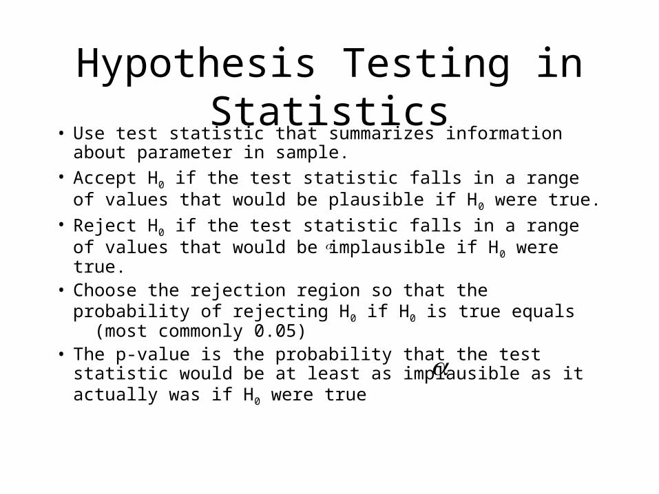
Hypothesis Testing in Statistics• Use test statistic that summarizes information about

parameter in sample.• Accept H0 if the test statistic falls in a range of values that

would be plausible if H0 were true.• Reject H0 if the test statistic falls in a range of values that

would be implausible if H0 were true.• Choose the rejection region so that the probability of

rejecting H0 if H0 is true equals (most commonly 0.05)• The p-value is the probability that the test statistic would be

at least as implausible as it actually was if H0 were true

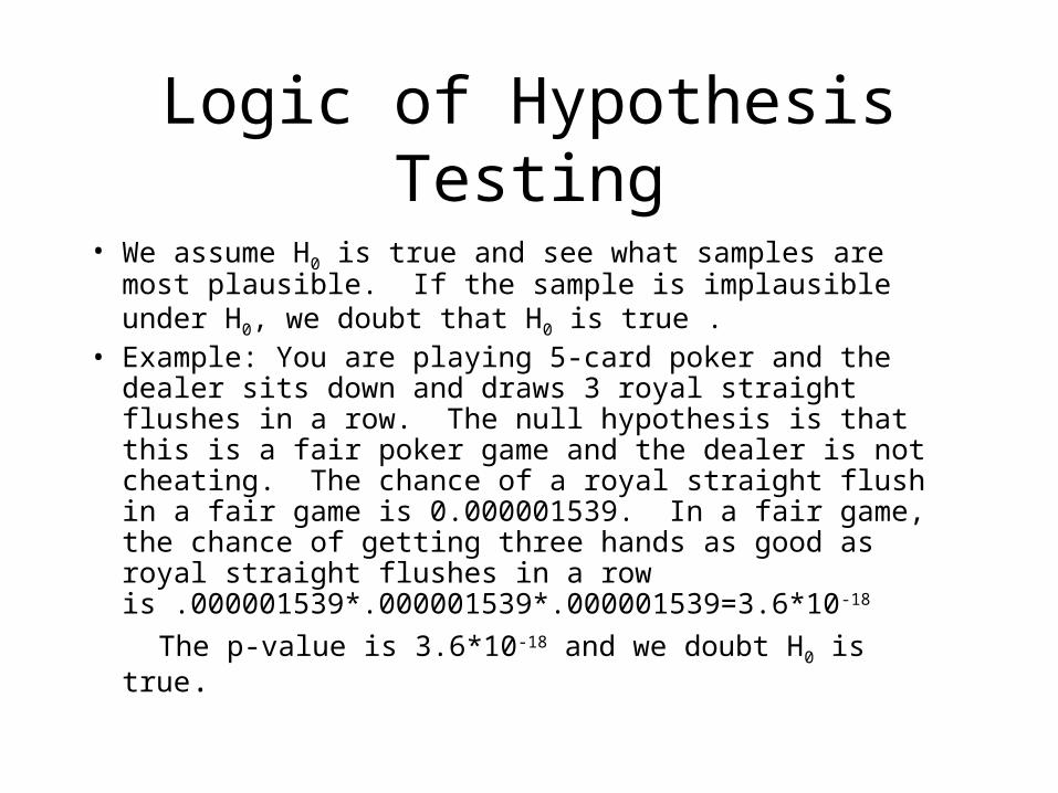
Logic of Hypothesis Testing

• We assume H0 is true and see what samples are most plausible. If the sample is implausible under H0, we doubt that H0 is true .

• Example: You are playing 5-card poker and the dealer sits down and draws 3 royal straight flushes in a row. The null hypothesis is that this is a fair poker game and the dealer is not cheating. The chance of a royal straight flush in a fair game is 0.000001539. In a fair game, the chance of getting three hands as good as royal straight flushes in a row is .000001539*.000001539*.000001539=3.6*10-18

The p-value is 3.6*10-18 and we doubt H0 is true.

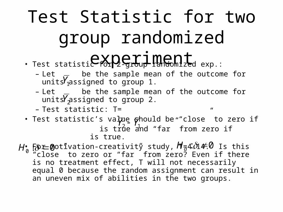
Test Statistic for two group randomized experiment

• Test statistic for 2-group randomized exp.:– Let be the sample mean of the outcome for units assigned

to group 1. – Let be the sample mean of the outcome for units assigned

to group 2.– Test statistic: T=

• Test statistic’s value should be “close” to zero if is true and “far” from zero if is true. • For motivation-creativity study, T=4.14. Is this “close” to zero

or “far” from zero? Even if there is no treatment effect, T will not necessarily equal 0 because the random assignment can result in an uneven mix of abilities in the two groups.

1Y

2Y

12 YY

0:0 H 0: aH

Randomization Test p-value

• The observed value of the test statistic can be extreme (far from zero) because– (a) there is an effect of the treatment

– (b) the random assignment resulted in an uneven mix

• A randomization test p-value is the probability associated with explanation (b)

• The smaller the p-value, the less believable (b) is as an explanation.

Exact Calculation of the p-value

• The p-value is the probability that |T|>=4.14 if, in fact, there is no treatment effect (and based on the random assignment of units to groups)

• Important starting point: If there is no treatment effect, then the creativity score for an individual would have been the same had they been assigned to the other group.

• Exact Calculation of p-value– Calculate T for every possible grouping of the 47 numbers

into groups of size 23 and 24– The p-value is the proportion of regroupings with |T|>=4.14.

Example

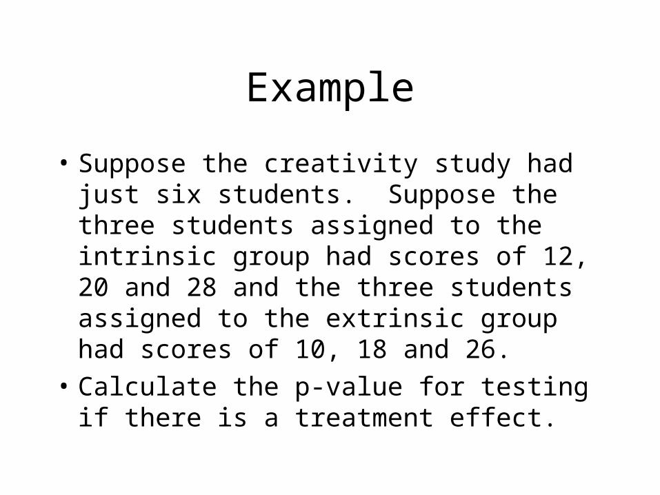
• Suppose the creativity study had just six students. Suppose the three students assigned to the intrinsic group had scores of 12, 20 and 28 and the three students assigned to the extrinsic group had scores of 10, 18 and 26.

• Calculate the p-value for testing if there is a treatment effect.

P-value for Creativity Study

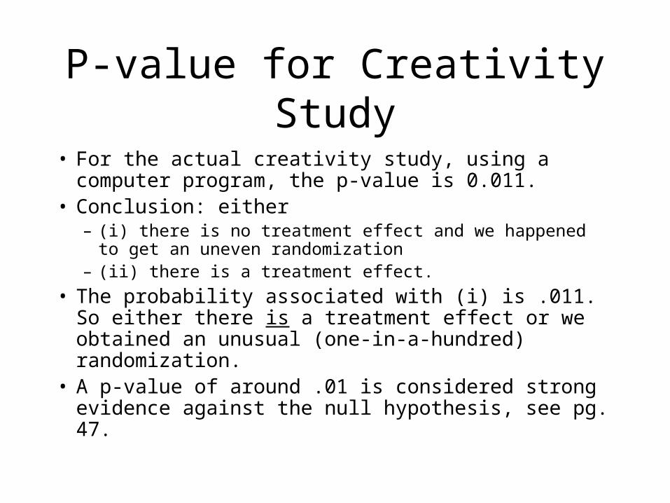
• For the actual creativity study, using a computer program, the p-value is 0.011.

• Conclusion: either– (i) there is no treatment effect and we happened to get an

uneven randomization– (ii) there is a treatment effect.

• The probability associated with (i) is .011. So either there is a treatment effect or we obtained an unusual (one-in-a-hundred) randomization.

• A p-value of around .01 is considered strong evidence against the null hypothesis, see pg. 47.

Approximating the p-value

• For the creativity study, there are 1.6*1013 different groupings.

• Approximating the randomization test p-value.– (i) Monte Carlo simulation: Randomly choose many

groupings. Approximate the randomization distribution by the histogram of the test statistic for the randomly chosen groupings

– (ii) (Chapter 2). The randomization distribution of the “t-statistic” is approximated by the “t”-distribution.

Decisions based on p-values

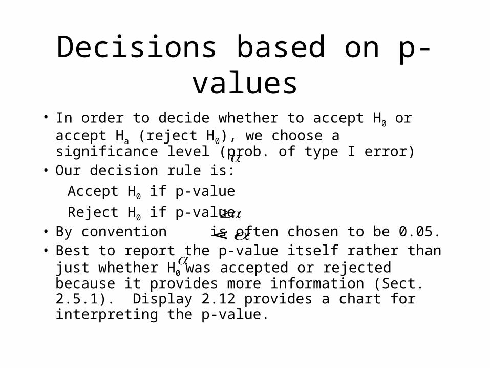
• In order to decide whether to accept H0 or accept Ha (reject H0), we choose a significance level (prob. of type I error)

• Our decision rule is:

Accept H0 if p-value

Reject H0 if p-value • By convention is often chosen to be 0.05.• Best to report the p-value itself rather than just whether H0

was accepted or rejected because it provides more information (Sect. 2.5.1). Display 2.12 provides a chart for interpreting the p-value.

One-sided vs. Two-sided Tests

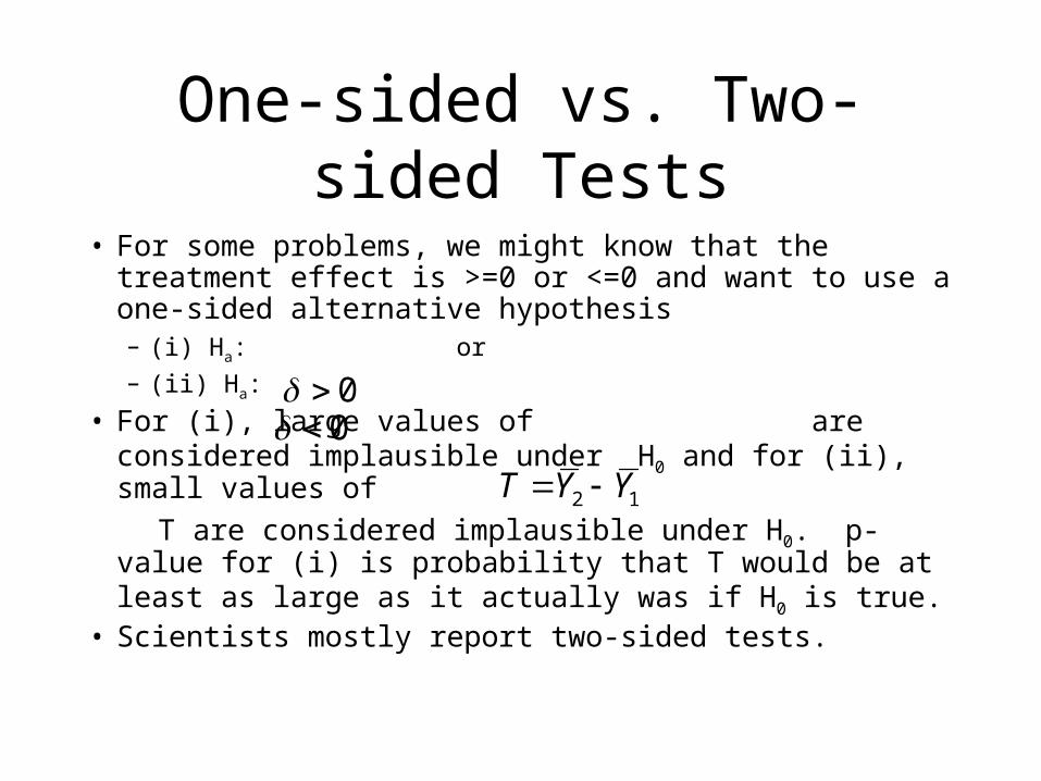
• For some problems, we might know that the treatment effect is >=0 or <=0 and want to use a one-sided alternative hypothesis– (i) Ha: or – (ii) Ha:

• For (i), large values of are considered implausible under H0 and for (ii), small values of

T are considered implausible under H0. p-value for (i) is probability that T would be at least as large as it actually was if H0 is true.

• Scientists mostly report two-sided tests.

00

12 YYT

Scope of Inference

• The conclusion that the intrinsic questionnaire causes a difference in creativity (i.e., ) strictly applies only to the subjects in the study. If the subjects were obtained by a random sample, then we could conclude that the intrinsic questionnaire has causal effects for a larger population (see Display 1.5).

0

The meaning of the causal inference

• In the motivation-creativity study, we concluded that there is a strong evidence that the “intrinsic questionnaire” treatment caused a difference in creativity compared to the “extrinsic questionnaire” treatment.

• This difference could be caused by anything that differs between the two treatments, e.g, the actual questionnaire, the order in which the poems were judged, the relative preferences of the judges for the two treatments.

Control in Experimental Design

• The principle of control in experimental design is to make sure that all other factors besides the intended treatments are kept the same in the different groups. Then we conclude that the intended treatment causes a difference between the groups.

• Examples of control:– Use a placebo for the control group.– Double blinding– Judge poems in random order.

Experimental Design Example: Salk Vaccine Field Trial

• In the first half of the 20th century, polio was one of the most frightening diseases, striking hardest at young children and leaving many helpless cripples.

• By the 1950s, Jonas Salk developed a vaccine for polio that had proved promising in laboratory experiments but it was necessary to try it in the real world before releasing it for general use.

Designs for Salk Vaccine Field Trial

• Historical Control Approach: Distribute the vaccine as widely as possible, through the schools, to see whether the rate of reported polio was appreciably less than usual during the subsequent season.

• Observed Control Approach: Offer vaccination to all children in the second grade of participating schools and follow the polio experience not only in these children but in the first and third grade children.

• Placebo Control Approach: Choose the control group from the same population as the treatment group – children whose parents consented to vaccination. Assign the treatment randomly. Give a placebo to control group. Do not tell doctors which group children belong to.