Lecture 3: Informed (Heuristic) Searchdprecup/courses/AI/Lectures/ai-lecture03.pdf• If the...

Lecture 3: Informed (Heuristic) Search

• Best-First (Greedy) Search

• Heuristic Search

• A∗ search

• Proof of optimality of A∗

• Variations: iterative deepening, real-time search, macro-actions

COMP-424, Lecture 3 - January 14, 2013 1

Recall from last time: General search

!"#$%&'(&#)$*$&$+,-./$*&*&0*&12*#&,&*#,#$3&("#&($4$**,50/6&,&*#,5#&*#,#$

7

8"9&:"$*&;<=&$+.,(:>&8"9&:"&6"2&:$40:$&9)04)&($+#&(":$>&&?*$&,&

*#,4@A$+.,(:&#)$&*#,#$*&-"*#&5$4$(#/6&,::$:&#"&#)$&*#,4@B

8"9&:"$*&C<=&$+.,(:>&?*$&,&D2$2$A$+.,(:&#)$&*#,#$*&#),#&9$5$&,::$:&E05*#&#"&

#)$&D2$2$B

• Problems are described through states, operators and costs• For each state and operator, there is a set of successor states• In search, we maintain a set of nodes, each containing a state and otherinfo (e.g. cost so far, pointer to parent etc)

• These nodes form a search tree• The fringe of the tree contains candidate nodes, and is typicallymaintained using a priority queue

• Different search algorithms use different priority functions f


Uninformed vs. informed search

• Uninformed search methods expand nodes based on the distance fromthe start node. Obviously, we always know that!

• Informed search methods also use some estimate of the distance to thegoal h(n), called a heuristic.

• If we knew the distance to goal exactly, it would not even be “search” -we could just be greedy!

• But even if we do not know the exact distance, we often have someintuition about this distance:

– The straight line between two points, in a navigation problem– The number of misplaced tiles in the 8-puzzle

• The heuristic is often the result of thinking about a relaxed version ofthe problem.


Best-First Search

• Algorithm: At any time, expand the most promising node according tothe heuristic

• This is roughly the “opposite” of uniform-cost search

• Example:

!"#"#$%&'$('##)*$+,-$./$/0&123$42)$1#$4514*/$647#$60#$5&1#/6$0$845"#9$$:460$./$

;<

%.'/6$2&)#$.2$#4=0$/6#>$.%$/&'6#)$?*$?#/6$0#"'./6.=9

+"6$60./$./2@6$60#$/0&'6#/6$>460$.2$6#'A/$&%$=&/69$$-&$(+,-$2&6$&>6.A453$#8#2$60&"B0$

0#"'./6.=$%"2=6.&2$./$CB&&)D9

E$4514*/$F"2)#'#/6.A46#/F$/0&'6#/6$>460$6&$B&459

+"6$(+,-$./$8#'*$#4/*$6&$.A>5#A#263$42)$60#'#$4'#$>'&?5#A/$%&'$10.=0$.6$./$B'#469

At node A, we choose to go to node C, because it has a better heuristicvalue, instead of not B, which is really optimal


Properties of best-first search

• Time complexity: O(bd) (where b is the branching factor and d is thedepth of the solution)

• If the heuristic is always 0, best-first search is the same as breadth-firstsearch - so in the worst-case, it will have exponential space complexity

• However, depending on the heuristic, the expansion may look a lot likedepth-first search - so space complexity may look like O(bd).

• Like DFS, best-first search is not complete in general

– Can go on forever in infinite state space– In finite state space, can get stuck in loops unless we use a closed list

• Not optimal! (as seen in the example)

• Best-first search is a greedy method.

Greedy methods maximize short-term advantage without worrying aboutlong-term consequences.


Fixing greedy search

• The problem with best-first search is that it is too greedy: it does nottake into account the cost so far!

• Let g be the cost of the path so far

• Let h be a heuristic function (estimated cost to go)

• Heuristic search is a best-first search, greedy with respect to

f = g + h

• Important insight: f = g + h as an estimate of the cost of the currentpath


Heuristic Search Algorithm

• At every step:

1. Dequeue node n from the front of the queue2. Enqueue all its successors n� with priorities:

f(n�) = g(n�) + h(n�)

= cost of getting to n� + estimated cost from n

� to goal

3. Terminate when a goal state is popped from the queue.

• Does this work on our previous example?

!"#"#$%&'$('##)*$+,-$./$/0&123$42)$1#$4514*/$647#$60#$5&1#/6$0$845"#9$$:460$./$

;<

%.'/6$2&)#$.2$#4=0$/6#>$.%$/&'6#)$?*$?#/6$0#"'./6.=9

+"6$60./$./2@6$60#$/0&'6#/6$>460$.2$6#'A/$&%$=&/69$$-&$(+,-$2&6$&>6.A453$#8#2$60&"B0$

0#"'./6.=$%"2=6.&2$./$CB&&)D9

E$4514*/$F"2)#'#/6.A46#/F$/0&'6#/6$>460$6&$B&459

+"6$(+,-$./$8#'*$#4/*$6&$.A>5#A#263$42)$60#'#$4'#$>'&?5#A/$%&'$10.=0$.6$./$B'#469


Example

6

S

A B

C

G

1 1

h=6

7

h=3

h=2

2

Priority queue: (S,h(S))


Example

6

S

A B

C

G

1 1

h=6

7

h=3

h=2

2

Priority queue: ((B,4),(A,7))


Example

6

S

A B

C

G

1 1

h=6

7

h=3

h=2

2

Priority queue: ((C,5),(A,7))


Example

6

S

A B

C

G

1 1

h=6

7

h=3

h=2

2

Priority queue: ((A,7), (G,9))


Example

6

S

A B

C

G

1 1

h=6

7

h=3

h=2

2

Priority queue: ((G,8), (G,9)) ⇒ the optimal path through A is found!


Does heuristic search always give the optimal solution?

S

A

G

1

1

3

• Whether the solution is optimal depends on the heuristic

• E.g., in the example above, any value of h(A) ≥ 3 will lead to thediscovery of a suboptimal path

• Can we put conditions on the choice of heuristic to guarantee optimality?


Admissible heuristics

• Let h∗(n) be the shortest path from n to any goal state.

• Heuristic h is called admissible if h(n) ≤ h∗(n)∀n.• Admissible heuristics are optimistic

• Note that if h is admissible, then h(g) = 0, ∀g ∈ G

• A trivial case of an admissible heuristic is h(n) = 0, ∀n.– In this case, heuristic search becomes uniform-cost search!


Examples of admissible heuristics

• Robot navigation: straight-line distance to goal

• 8-puzzle: number of misplaced tiles

• 8-puzzle: sum of Manhattan distances for each tile to its goal position(why?)

• In general, if we get a heuristic by solving a relaxed version of a problem,we will obtain an admissible heuristic (why?)


A∗search

• Heuristic search with an admissible heuristic!

• Let g be the cost of the path so far

• Let h be an admissible heuristic function

I.e. h is optimistic, it never overestimates the actual cost to the goal

• Do a greedy search with respect to

f = g + h


A∗Pseudocode

1. Initialize the queue with (S, f(S)), where S is the start state

2. While queue is not empty:

(a) Pop node n with lowest priority from the priority queue; let s be theassociated state and f(s) the associated priority value

(b) If s is a goal state, return success (follow back pointers from n toextract best path)

(c) Else, for all states s� ∈ Successor(s)i. Compute f(s�) = g(s�) + h(s�) = g(s) + cost(s, s�) + h(s�)ii. If s� was previously expanded and the new f(s�) is smaller, or if s�

has not been expanded, or if s� is already in the queue, then createnode n� with priority f(s�) and insert it in the queue; else do nothing


Consistency

• An admissible heuristic h is called consistent if for every state s and forevery successor s�,

h(s) ≤ c(s, s�) + h(s�)

• This is a version of triangle inequality, so heuristics that respect thisinequality are metrics.

• If you think of h as estimating “distance to the goal”, it is quitereasonable to assume this property

• Note that if h is monotone, and all costs are non-zero, then f cannotdecrease along any path:

f(s) = g(s) + h(s) ≤ g(s) + c(s, s�) + h(s�) = f(s�)


Is A∗complete?

• Suppose that h is monotone ⇒ f is non-decreasing

• Note that in this case, a node cannot be re-expanded

• If a solution exists, it must have bounded cost

• Hence A∗ will have to find it! So it is complete


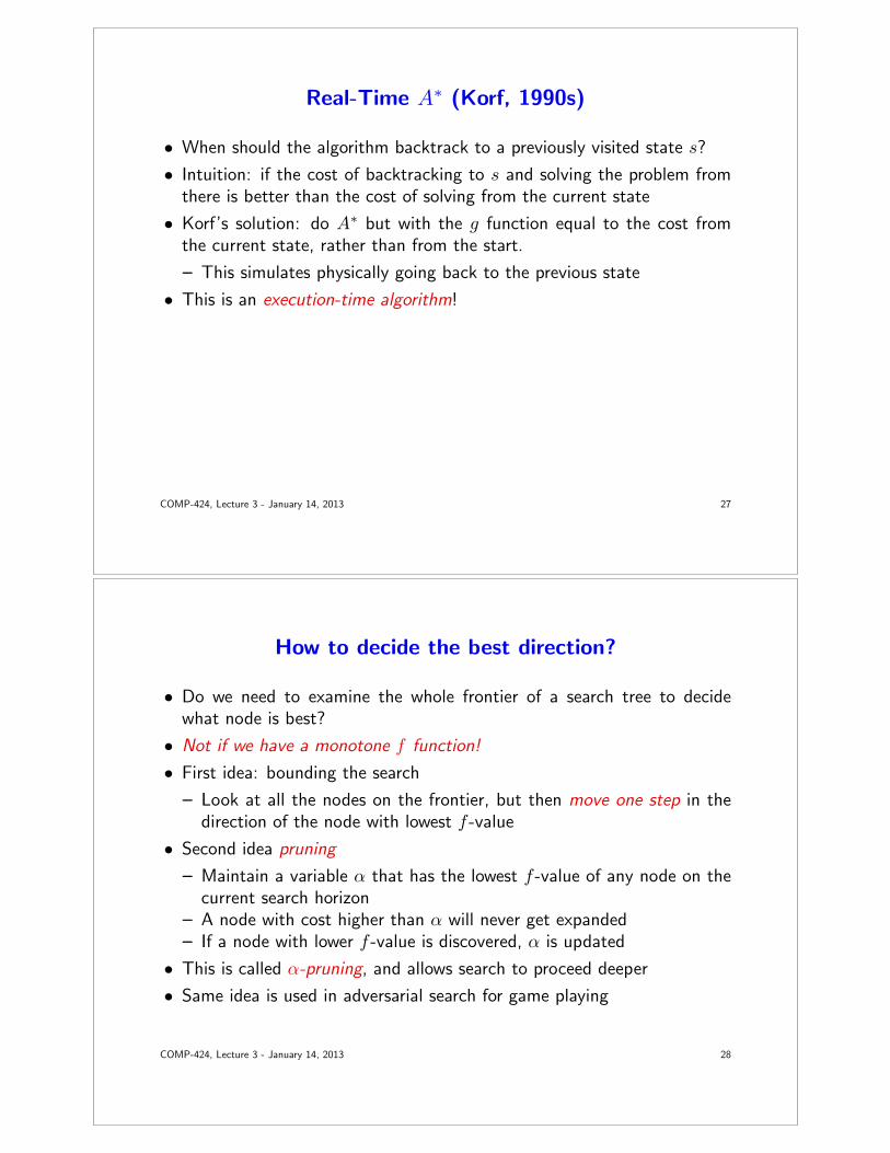
Dealing with inconsistent heuristics

n

n’

1

g=5, h=4, f=9

g’=6, h’=2, f’=8

• Make a small change to A∗: instead of f(s�) = g(s�) + h(s�), usef(s�) = max(g(s�) + h(s�), f(s))

• With this change, f is non-decreasing along any path, and the previousargument applies


Is A∗search optimal?

• Suppose some suboptimal node containing a goal state has beengenerated and is in the queue (call this node G2).

• Let n be an unexpanded node on a shortest optimal path, and call theend point of this path node G1.

• We have:

f(G2) = g(G2) since h(G2) = 0

> g(G1) since G2 is suboptimal

≥ f(n) since h is admissible

• Since f(G2) > f(n), A∗ will select n for expansion before G2

• Since n was chosen arbitrarily, all nodes on the optimal path will bechosen before G2, so G1 will be reached before G2


Dominance

• If h2(n) ≥ h1(n) for all n (both admissible) then h2 dominates h1

• A∗ using h1 will expand all nodes expanded when using h2, and more

• Eight-puzzle typical search example:

d = 14 IDS = 3,473,941 nodesA∗(h1) = 539 nodesA∗(h2) = 113 nodes

d = 24 IDS = too many nodesA∗(h1) = 39,135 nodesA∗(h2) = 1,641 nodes


Properties of A∗

• Complete!

• Optimal!

• Exponential worst-case time and space complexity (why?)

– But with a perfect heuristic, the complexity is O(bd), because wewould only expand the nodes along the optimal path

– With a good heuristic complexity is often sub-exponential

• Optimally efficient: with a given h, no other search algorithm will beable to expand fewer nodes


Iterative Deepening A∗(IDA∗

)

• Same trick as we used in last lecture to avoid memory problems

• The algorithm is basically depth-first search, but using the f -value todecide in which order to consider the descendents of a node

• There is an f -value limit, rather than a depth limit, and we expand allnodes up to f1, f2, . . .

• Additionally, we keep track of the next limit to consider (so we will searchat least one more node next time)

• IDA∗ has the same properties as A∗ but uses less memory

• In order to avoid expanding new nodes always, old ones can beremembered, if memory permits (a version know as SMA∗)


Iterative deepening example:

6

S

A B

C

G

1 1

h=6

7

h=3

h=2

2

• Set f1 = 4 −→ only S, B are searched (no other nodes are put in thequeue, because they exceed the cutoff threshold)

• Set f2 = 8 −→ now S, A, B, C, G are all searched


Real-Time Search

• In dynamic environments, agents have to act before they finish thinking!

• So instead of searching for a complete path to goal, we would like theagent to do a bit of search, then move in the direction of the currently“best” path

• Main issue: how do we avoid cycles, if we do not have enough memoryto mark states?


Real-Time A∗(Korf, 1990s)

• When should the algorithm backtrack to a previously visited state s?

• Intuition: if the cost of backtracking to s and solving the problem fromthere is better than the cost of solving from the current state

• Korf’s solution: do A∗ but with the g function equal to the cost fromthe current state, rather than from the start.

– This simulates physically going back to the previous state

• This is an execution-time algorithm!


How to decide the best direction?

• Do we need to examine the whole frontier of a search tree to decidewhat node is best?

• Not if we have a monotone f function!

• First idea: bounding the search

– Look at all the nodes on the frontier, but then move one step in thedirection of the node with lowest f -value

• Second idea pruning

– Maintain a variable α that has the lowest f -value of any node on thecurrent search horizon

– A node with cost higher than α will never get expanded– If a node with lower f -value is discovered, α is updated

• This is called α-pruning, and allows search to proceed deeper

• Same idea is used in adversarial search for game playing


Search improvements

• Consider Rubik’s cube: 43,252,003,274,489,856,000 states!

• How do people solve this puzzle?


Changing the search problem

• People do not think at the level of individual moves!• Instead, there are sequences of moves, designed to achieve a certainpattern (L-shape, fish, etc)

• Instead of choosing individual operators, you choose what subgoal youwant to achieve next

• Then solve the subgoal, and choose the next subgoal• Often the solution to a subgoal is quite standard (e.g a fish on any cornercan be achieved in a similar way)


Abstraction and decomposition

• The key to solving complicated problems is to decompose them intosmaller parts

• Each part may be easy to solve; then we put the solutions together

• Abstraction is a term used to refer to methods that choose to ignoreinformation, in order to speed up computation

E.g. in Rubik’s cube, we focus only on a certain aspect of the state, likethe fish, and ignore the rest of the tiles!

• Intuitively, abstraction means that we construct a smaller problem, inwhich many states of the original problem are mapped to a single abstractstate

• A macro-action is a sequence of actions from the original problem (thinklarge jump)

– E.g. Swapping two tiles in the 8-puxxle– E.g. Making a T in Rubik’s cube


Example: Landmark navigation

• Find a path from the current location to a well-known landmark (e.g.McGill metro)

• Find a path between landmarks (this can even be pre-computed!)

• Find a pat from last landmark to destination


Trade-offs

• By decomposing a problem and putting the solutions together, we maybe giving up optimality

• But otherwise we may not be able to solve the problem at all!

• Solutions to subgoals are often cached in a database

• When we choose subgoals, we need to be careful that the overall problemstill has a solution

– Knoblock (1990s) showed conditions under which sub-solutions canbe pieced together an completeness is preserved


Summary of informed search

• Insight: use knowledge about the problem, in the form of a heuristic.

– The heuristic is a guess for the remaining cost to the goal.– A good heuristic can reduce the search time from exponential to

almost linear.

• Best-first search is greedy with respect to the heuristic, not completeand not optimal

• Heuristic search is greedy with respect to f = g + h, where g is the costso far and h is the estimated cost to go

• A∗ is heuristic search where h is an admissible heuristic; it is completeand optimal

• A∗ is a key AI search algorithm


Lecture 3: Informed (Heuristic) Searchdprecup/courses/AI/Lectures/ai-lecture03.pdf• If the...

Documents

Transcript of Lecture 3: Informed (Heuristic) Searchdprecup/courses/AI/Lectures/ai-lecture03.pdf• If the...