Lecture 3 April 22, 2013 - Emerson Statistics
93
Lecture 3 April 22, 2013 Statistical Design of Clinical Trials, SPR 2013 Biost 578A: Special Topics Statistical Design of Clinical Trials Scott S. Emerson, M.D., Ph.D. Professor of Biostatistics University of Washington Lecture 3: Sequential Sampling April 22, 2013 Introduction to RCTdesign 3 Chronology • 1987 – 1995 Research software – Design of GST, estimation following GST • 1995 Review of PEST, East for The American Statistician – Little overlap of designs – Inadequate evaluation (especially in East at the time) • 1995 – 2000 SBIR to MathSoft (Insightful Tibco) – S+SeqTrial • 2002 – 2006 Extensions • 2010 – 2011 RCTdesign: Porting S+SeqTrial functionality to R • 2012 – 20?? Continued extensions 4 RCTdesign: Raison d’Etre • Software for design, conduct, and analysis of sequential clinical trials – A broad spectrum of group sequential designs – A full complement of tools for evaluation of operating characteristics – Seamless progression from design to monitoring to analysis • Extensible, object-oriented language to facilitate – Exploration of alternative designs to address needs of individual trials – Research into development of new clinical trial methodology
Transcript of Lecture 3 April 22, 2013 - Emerson Statistics
Lecture 3 April 22, 2013
Statistical Design of Clinical Trials, SPR 2013
Biost 578A: Special TopicsStatistical Design of Clinical Trials
Scott S. Emerson, M.D., Ph.D.Professor of BiostatisticsUniversity of Washington
Lecture 3:Sequential Sampling
April 22, 2013
Introduction to RCTdesign
3
Chronology
• 1987 – 1995 Research software– Design of GST, estimation following GST
• 1995 Review of PEST, East for The American Statistician– Little overlap of designs– Inadequate evaluation (especially in East at the time)
• 1995 – 2000 SBIR to MathSoft (Insightful Tibco)– S+SeqTrial
• 2002 – 2006 Extensions
• 2010 – 2011 RCTdesign: Porting S+SeqTrial functionality to R
• 2012 – 20?? Continued extensions4
RCTdesign: Raison d’Etre
• Software for design, conduct, and analysis of sequential clinical trials– A broad spectrum of group sequential designs– A full complement of tools for evaluation of operating
characteristics– Seamless progression from design to monitoring to analysis
• Extensible, object-oriented language to facilitate– Exploration of alternative designs to address needs of individual
trials– Research into development of new clinical trial methodology

Lecture 3 April 22, 2013
Statistical Design of Clinical Trials, SPR 2013
5
The Problem of Clinical Trial Design
Happy families are all alike; every unhappy family is unhappy in its own way.
Leo Tolstoy, Anna Karenina, 1873-77
6
The Problem of Clinical Trial Design
Unbiased clinical trials are all alike; every biased clinical trial is biased in its own way.
7
Clinical Trial Design
• Finding an approach that best addresses the often competing goals: Science, Ethics, Efficiency– Basic scientists: focus on mechanisms– Clinical scientists: focus on overall patient health– Ethical: focus on patients on trial, future patients– Economic: focus on profits and/or costs– Governmental: focus on safety of public: treatment safety,
efficacy, marketing claims– Statistical: focus on questions answered precisely – Operational: focus on feasibility of mounting trial
8
Statistical Planning
• Satisfy collaborators as much as possible
• Discriminate between relevant scientific hypotheses– Scientific and statistical credibility
• Protect economic interests of sponsor– Efficient designs– Economically important estimates
• Protect interests of patients on trial– Stop if unsafe or unethical– Stop when credible decision can be made
• Promote rapid discovery of new beneficial treatments

Lecture 3 April 22, 2013
Statistical Design of Clinical Trials, SPR 2013
9
Classical Fixed Sample Designs
• Design stage: – Choose a sample size
• Conduct stage: – Recruit subjects, gather all the data
• Analysis stage: – When all data available, analyze and report
10
Statistical Sampling Plan
• Ethical and efficiency concerns are addressed through sequential sampling
• During the conduct of the study, data are analyzed at periodic intervals and reviewed by the DMC
• Using interim estimates of treatment effect– Decide whether to continue the trial
• Stop if scientifically relevant and statistically credible results have been obtained
– If continuing, decide on any modifications to • sampling scheme• scientific / statistical hypotheses and/or
11
Ultimate Goal
• Modify the sample size accrued so that minimal number of subjects treated when– new treatment is harmful,– new treatment is minimally effective, or– new treatment is extremely effective
• Only proceed to maximal sample size when– not yet certain of treatment benefit, or– potential remains that results of clinical trial will eventually lead
to modifying standard practice
12
Group Sequential Designs
• Design stage: – Choose an interim monitoring plan– Choose a maximal stopping time
• Statistical information, sample size, calendar time
• Conduct stage: – Recruit subjects, gather data in groups– After each group, analyze for DMC
• DMC recommends termination or continuation
• Analysis stage: – When study stops, analyze and report

Lecture 3 April 22, 2013
Statistical Design of Clinical Trials, SPR 2013
13
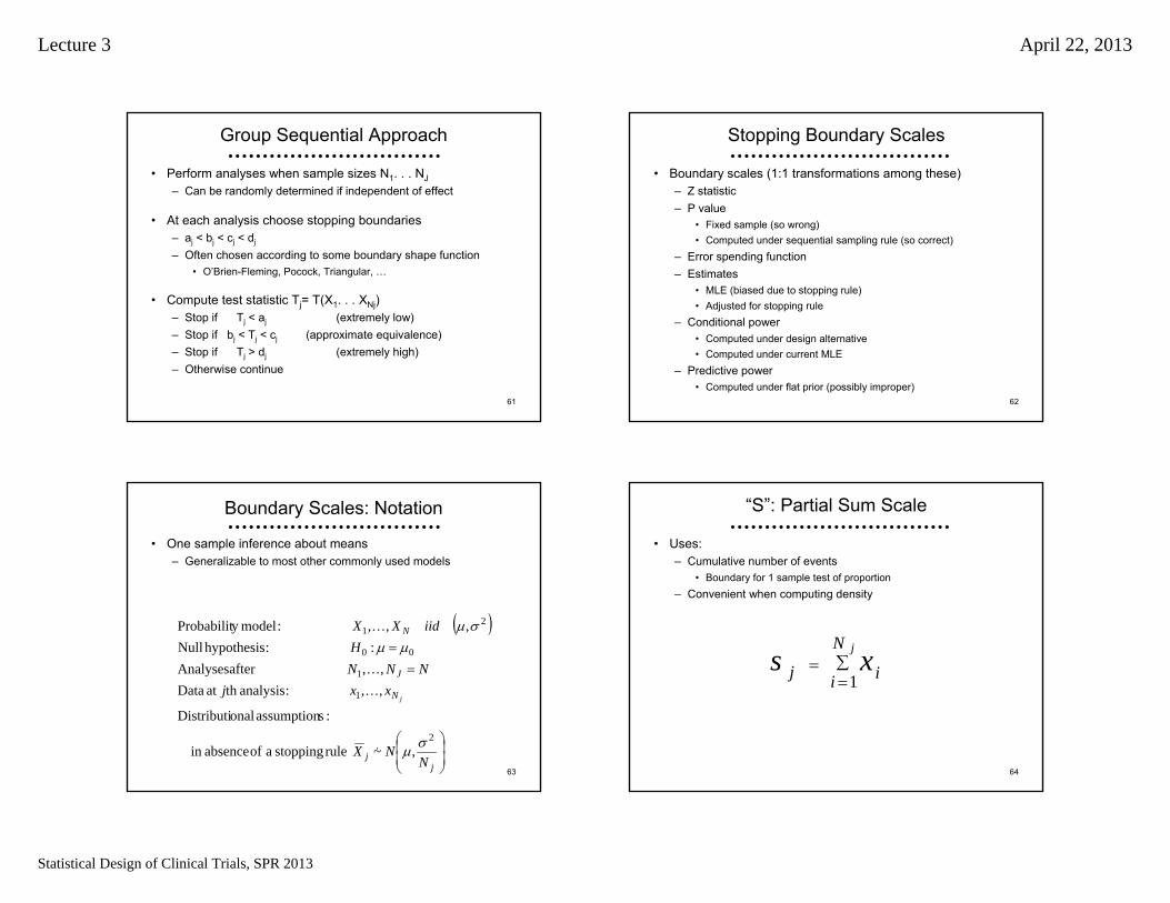
Group Sequential Approach
• Perform analyses when sample sizes N1. . . NJ– Can be randomly determined if independent of effect
• At each analysis choose stopping boundaries– - < aj < bj < cj < dj <
• Compute test statistic Tj= T(X1. . . XNj)– Stop if Tj < aj (extremely low)– Stop if bj < Tj < cj (approximate equivalence)– Stop if Tj > dj (extremely high)– Otherwise continue
• Special cases– Definitely stop if aj = bj and cj = dj
– No stopping if aj = - and bj = cj and dj = 14
Group Sequential Sampling Distribution
• Perform analyses when sample sizes N1. . . NJ– Can be randomly determined if independent of effect
• At each analysis choose continuation sets– Cj = (aj , bj ] [ cj , dj )
• Compute test statistic Tj= T(X1. . . XNj)– Stop if Tj Cj
– Otherwise continue
• (The decision associated with stopping does not affect the sampling distribution.)
15
Statistical Design Issues
• Under what conditions should we use fewer subjects?– Ethical treatment of patients– Efficient use of resources (time, money, patients)– Scientifically meaningful results– Statistically credible results– Minimal number of subjects for regulatory agencies
• How do we control false positive rate?– Repeated analysis of accruing data involves multiple
comparisons
16
Sample Path for a Statistic

Lecture 3 April 22, 2013
Statistical Design of Clinical Trials, SPR 2013
17
Fixed Sample Methods Wrong
• Simulated trials using Z < -1.96 or Z > 1.96
18
If Only a Single Analysis…
• Simulated trials: 1 of 20 significant at final analysis– True type I error: 0.05
19
If Early Stopping at Nominal 0.05 Level
• Simulated trials under null stop too often: 6 of 20– True type I error: 0.1417
20
100,000 Simulated Trials (Pocock)
• Three equally spaced level .05 analysesPattern of Proportion SignificantSignificance 1st 2nd 3rd Ever
1st only .03046 .030461st, 2nd .00807 .00807 .008071st, 3rd .00317 .00317 .003171st, 2nd, 3rd .00868 .00868 .00868 .008682nd only .01921 .019212nd, 3rd .01426 .01426 .014263rd only .02445 .02445
Any pattern .05038 .05022 .05056 .10830

Lecture 3 April 22, 2013
Statistical Design of Clinical Trials, SPR 2013
21
100,000 Simulated Trials (Pocock)
• Three equally spaced level .05 analysesPattern of Proportion SignificantSignificance 1st 2nd 3rd Ever
1st only .03046 .030461st, 2nd .00807 .00807 .008071st, 3rd .00317 .00317 .003171st, 2nd, 3rd .00868 .00868 .00868 .008682nd only .01921 .019212nd, 3rd .01426 .01426 .014263rd only .02445 .02445
Any pattern .05038 .05022 .05056 .10830
22
100,000 Simulated Trials (Pocock)
• Three equally spaced level .05 analysesPattern of Proportion SignificantSignificance 1st 2nd 3rd Ever
1st only .03046 .030461st, 2nd .00807 .00807 .008071st, 3rd .00317 .00317 .003171st, 2nd, 3rd .00868 .00868 .00868 .008682nd only .01921 .019212nd, 3rd .01426 .01426 .014263rd only .02445 .02445
Any pattern .05038 .05022 .05056 .10830
23
Pocock Level 0.05
• Three equally spaced level .022 analysesPattern of Proportion SignificantSignificance 1st 2nd 3rd Ever
1st only .01520 .015201st, 2nd .00321 .00321 .003211st, 3rd .00113 .00113 .001131st, 2nd, 3rd .00280 .00280 .00280 .002802nd only .01001 .010012nd, 3rd .00614 .00614 .006143rd only .01250 .01250
Any pattern .02234 .02216 .02257 .05099
24
Unequally Spaced Analyses
• Level .022 analyses at 10%, 20%, 100% of dataPattern of Proportion SignificantSignificance 1st 2nd 3rd Ever
1st only .01509 .015091st, 2nd .00521 .00521 .005211st, 3rd .00068 .00068 .000681st, 2nd, 3rd .00069 .00069 .00069 .000692nd only .01473 .014732nd, 3rd .00165 .00165 .001653rd only .01855 .01855
Any pattern .02167 .02228 .02157 .05660

Lecture 3 April 22, 2013
Statistical Design of Clinical Trials, SPR 2013
25
Varying Critical Values (O’Brien-Fleming)
• =0.10; equally spaced using naïve .003, .036, .087Pattern of Proportion SignificantSignificance 1st 2nd 3rd Ever
1st only .00082 .000821st, 2nd .00036 .00036 .000361st, 3rd .00037 .00037 .000371st, 2nd, 3rd .00127 .00127 .00127 .001272nd only .01164 .011642nd, 3rd .02306 .02306 .023063rd only .06223 .01855
Any pattern .00282 .03633 .08693 .09975
26
Error Spending: Pocock 0.05
Pattern of Proportion SignificantSignificance 1st 2nd 3rd Ever
1st only .01520 .015201st, 2nd .00321 .00321 .003211st, 3rd .00113 .00113 .001131st, 2nd, 3rd .00280 .00280 .00280 .002802nd only .01001 .010012nd, 3rd .00614 .00614 .006143rd only .01250 .01250
Any pattern .02234 .02216 .02257 .05099Incremental error .02234 .01615 .01250Cumulative error .02234 .03849 .05099
27
Distinctions without Differences
• Sequential sampling plans– Group sequential stopping rules– Error spending functions– Conditional / predictive power– Bayesian posterior probabilities
• Statistical treatment of hypotheses– Superiority / Inferiority / Futility– Two-sided tests / bioequivalence
28
Major Statistical Issue
• Frequentist operating characteristics are based on the sampling distribution
• Stopping rules do affect the sampling distribution of the usual statistics – MLEs are not normally distributed– Z scores are not standard normal under the null
• (1.96 is irrelevant)– The null distribution of fixed sample P values is not uniform
• (They are not true P values)
• Bayesian operating characteristics are based on the sampling distribution and a prior distribution– Is stopping rule relevant?

Lecture 3 April 22, 2013
Statistical Design of Clinical Trials, SPR 2013
29
Sampling Distribution of MLE
30
Sampling Distribution of MLE
31
Sampling Distributions
32
So What?
• Demystification: All we are doing is statistics– Planning a study
– Gathering data
– Analyzing it

Lecture 3 April 22, 2013
Statistical Design of Clinical Trials, SPR 2013
33
Sequential Studies
• Demystification: All we are doing is statistics– Planning a study
• Added dimension of considering time required– Gathering data
• Sequential sampling allows early termination– Analyzing it
• The same old inferential techniques• The same old statistics• But new sampling distribution
34
Familiarity and Contempt
• For any known stopping rule, however, we can compute the correct sampling distribution with specialized software– Standalone programs
• PEST (some integration with SAS)• EaSt
– Within statistical packages• S+SeqTrial• SAS PROC SEQDESIGN• R: gsDesign and RCTdesign (SeqTrial)
35
Sampling Density
• Armitage, McPherson, and Rowe (1969)– Sequential sampling density for normally distributed Xi
1
;,11;,
1;,1
1;,;,
, statistic Sequential
:min timeStopping
11
1
11
1
m
m
Cmm
mm
mm
Cx
M
jj
duumfNN
NuxNNN
xmf
NNxN
Nxf
xmfxmp
XM
CXjM
36
Familiarity and Contempt
• From the computed sampling distributions we then compute– Bias adjusted estimates– Correct (adjusted) confidence intervals– Correct (adjusted) P values
• Candidate designs can then be compared with respect to their operating characteristics

Lecture 3 April 22, 2013
Statistical Design of Clinical Trials, SPR 2013
37
Example: P Value
• Null sampling density tail
38
Evaluation of Designs
• Define candidate design constraining two operating characteristics– Type I error, power at design alternative– Type I error, maximal sample size
• Evaluate other operating characteristics– Sample size requirements– Power curve– Inference to be reported upon termination– (Probability of a reversed decision)
• Modify design
• Iterate
39
But What If …?
• Possible motivations for adaptive designs– Changing conditions in medical environment
• Approval / withdrawal of competing / ancillary treatments• Diagnostic procedures
– New knowledge from other trials about similar treatments
– Evidence from ongoing trial• Toxicity profile (therapeutic index)• Interim estimates of primary efficacy / effectiveness endpoint
– Overall– Within subgroups
• Interim alternative analyses of primary endpoints• Interim estimates of secondary efficacy / effectiveness endpoints
40
Adaptive Sampling Plans
• At each interim analysis, possibly modify statistical or scientific aspects of the RCT
• Primarily statistical characteristics– Maximal statistical information (UNLESS: impact on MCID)– Schedule of analyses (UNLESS: time-varying effects)– Conditions for stopping (UNLESS: time-varying effects)– Randomization ratios– Statistical criteria for credible evidence
• Primarily scientific characteristics– Target patient population (inclusion, exclusion criteria)– Treatment (dose, administration, frequency, duration)– Clinical outcome and/or statistical summary measure

Lecture 3 April 22, 2013
Statistical Design of Clinical Trials, SPR 2013
41
Adaptive Sampling: Examples
• Response adaptive modification of sample size– Proschan & Hunsberger (1995); Cui, Hung, & Wang (1999)
• Response adaptive randomization– Play the winner (Zelen, 1979)
• Adaptive enrichment of promising subgroups– Wang, Hung & O’Neill (2009)
• Adaptive modification of endpoints, eligibility, dose, …– Bauer & Köhne (1994); LD Fisher (1998)
42
Adaptive Sampling: Issues
• How do the newer adaptive approaches relate to the constraint of human experimentation and scientific method?
• Effect of adaptive sampling on trial ethics and efficiency– Avoiding unnecessarily exposing subjects to inferior treatments– Avoiding unnecessarily inflating the costs (time / money) of RCT
• Effect of adaptive sampling on scientific interpretation– Exploratory vs confirmatory clinical trials
• Effect of adaptive sampling on statistical credibility– Control of type I error in frequentist analyses– Promoting predictive value of “positive” trial results
43
Adaptive Sample Size Determination
• Design stage: – Choose an interim monitoring plan– Choose an adaptive rule for maximal sample size
• Conduct stage: – Recruit subjects, gather data in groups– After each group, analyze for DMC
• DMC recommends termination or continuation– After penultimate group, determine final N
• Analysis stage: – When study stops, analyze and report
44
Adaptive Sample Size Approach
• Perform analyses when sample sizes N1. . . NJ– N1. . . NJ-1 can be randomly determined indep of effect
• At each analysis choose stopping boundaries– aj < bj < cj < dj
• At N1. . . NJ-1 compute test statistic Tj= T(X1. . . XNj)– Stop if Tj < aj (extremely low)– Stop if bj < Tj < cj (approximate equivalence)– Stop if Tj > dj (extremely high)– Otherwise continue
• At NJ-1 determine NJ according to value of Tj

Lecture 3 April 22, 2013
Statistical Design of Clinical Trials, SPR 2013
45
When Stopping Rules Not Pre-specified
• Methods to control the type I error have been described for fully adaptive designs– Most popular: Preserve conditional error function from some
fixed sample or group sequential design– Can have loss of efficiency relative to pre-specified designs
• Recently methods to compute bias adjusted estimates and confidence intervals have been developed– Loss of precision relative to pre-specified designs
46
Scientific Design Issues
• Under what conditions should we alter our hypotheses?– Definition of a “Treatment Indication”
• Disease• Patient population• Definition of treatment (dose, frequency, ancillary treatments, …)• Desired outcome
• How do we control false positive rate?– Multiple comparisons across subgroups, endpoints
• How do we provide inference for Evidence Based Medicine?
47
Adaptive Sampling: Issues
“Make new friends, but don’t forget the old. One is silver and the other is gold”
- Children’s song
48
CDER/CBER Guidance on Adaptive Designs
• Recommendations for use of adaptive designs in confirmatory studies– Fully pre-specified sampling plans– Use well understood designs
• Fixed sample• Group sequential plans• Blinded adaptation
– For the time-being, avoid less understood designs• Adaptation based on unblinded data
• Adaptive designs may be of use in early phase clinical trials

Lecture 3 April 22, 2013
Statistical Design of Clinical Trials, SPR 2013
49
Perpetual Motion Machines
• A major goal of this course is to discern the hyperbole in much of the recent statistical literature– The need for adaptive clinical trial designs
• What can they do that more traditional designs do not?– The efficiency of adaptive clinical trial designs
• Has this been demonstrated?• Are the statistical approaches based on sound statistical
foundations?– “Self-designing” clinical trials
• When are they in keeping with our scientific goals?
50
Important Distinctions in this Course
• What aspects of the RCT are modified?– Statistical: Modify only the sample size to be accrued – Scientific: Possibly modify the hypotheses related to patient
population, treatment, outcomes
• Are all planned modifications described at design?– “Prespecified adaptive rules”: Investigators describe
• Conditions under which trial will be modified and• What those modification will consist of
– “Fully adaptive”: At each analysis, investigators are free to use current data to modify future conduct of the study
• When do the modifications take place?– Immediately: Potential to stop study at current analysis– Future stages of the RCT: Change plans for next analysis
Implementation in R
52
Actual Use
• We use RCTdesign to narrow the search for useful group sequential designs– Typically specify type I error and
• Design alternative and desired power OR• Design alternative and maximal sample size OR• Maximal sample size and desired power
– Search through a family of stopping boundaries• Alternative criteria for early stopping: null, alternative, both• Alternative degrees of “early conservatism”• Alternative number and schedule of analyses
• We use RCTdesign to evaluate operating characteristics– Different operating characteristics of interest to differenct
collaborating disciplines

Lecture 3 April 22, 2013
Statistical Design of Clinical Trials, SPR 2013
53
Implementation in R: Basic Objects
• seqModel– Probability model for primary endpoint– Statistical analysis model
• seqBoundary– A stopping rule (on some scale)
• seqOperatingChar– Stopping probabilities– Power (including type I error)– Sample size distribution
• seqInference– Point estimates, confidence intervals, P values
54
Implementation in R: High Level Objects
• seqDesign– Probability model for primary endpoint– Statistical hypotheses– Design parameters to specify a boundary– Stopping boundaries
• seqMonitor– A group sequential design– Interim data– Updated monitoring boundaries– Statistical inference
55
Implementation in R: Operations
• Creation of objects– User interface to facilitate scientific interpretations– (Graphical user interface (GUI) under development)
• Printing objects– Information necessary for protocols, statistical analysis plans
• Plotting objects– Facilitate comparisons among candidate designs
• Updates of objects
56
Basics: Probability Model
• The primary clinical outcome of a RCT is summarized by
• Common choices for in two arm studies– Difference (or ratio) of means– Ratio of geometric means– Difference (or ratio) of proportions having some event– Ratio of odds of having some event– Ratio (or difference) or rates of some event– Ratio of hazards (time averaged?)
• Note that all of the above can be analyzed in (nearly) a distribution-free manner– Sums used in the statistics mean that CLT provides good
approximation

Lecture 3 April 22, 2013
Statistical Design of Clinical Trials, SPR 2013
57
Basics: Without Loss of Generality
• A one sample test of a one-sided hypothesis– Generalization to other probability models is immediate
• We will interpret our variability relative to average statistical info– Generalization to two sided hypothesis tests is straightforward
• Fixed sample one-sided tests– Test of a one-sided alternative (+ > 0 )
• Upper Alternative: H+: + (superiority) • Null: H0: 0 (equivalence, inferiority)
– Decisions based on some test statistic T:• Reject H0 (for H+) T c • Reject H+ (for H 0) T c
58
Basics: Notation
j
jNj
jNN
jNj
NN
iid
i
N
NVZZ
NVCov
NVN~
XX
VX
XXXX
j
jj
j
jj
J
/
ˆ :statistics test Interim
/ˆ,ˆ :increments Indep
/,ˆˆ :distn eApproximat
:sampling sequentialWithout
,,ˆˆ :estimates Interim
,~ :modely Probabilit
,,,, :data Potential
0
1
1
321
1
59
Basics: Without Loss of Generality
• Our ultimate interest is in comparing– Fixed sample tests– Group sequential tests– Other adaptive strategies
• We will thus further restrict attention to a one-sample setting in which– V = 1– Test of a one-sided alternative (+ > 0 )
• Upper Alternative: H+: + = 3.92 (superiority) • Null: H0: 0 = 0 (equivalence, inferiority)
60
Basics: Fixed Sample Test
• Sample size N = 1 provides– Type 1 error of 0.025– Power of 0.975 to detect the alternative of 3.92– At the final analysis, an observed estimate (or Z statistic) of 1.96
will be statistically significant
• Power and sample size table
1.000.9753.92
1.000.9003.24
1.000.8002.80
1.000.5001.96
1.000.0250.00
Avg NPowerTrue Effect
Lecture 3 April 22, 2013
Statistical Design of Clinical Trials, SPR 2013
61
Group Sequential Approach
• Perform analyses when sample sizes N1. . . NJ– Can be randomly determined if independent of effect
• At each analysis choose stopping boundaries– aj < bj < cj < dj
– Often chosen according to some boundary shape function• O’Brien-Fleming, Pocock, Triangular, …
• Compute test statistic Tj= T(X1. . . XNj)– Stop if Tj < aj (extremely low)– Stop if bj < Tj < cj (approximate equivalence)– Stop if Tj > dj (extremely high)– Otherwise continue
62
Stopping Boundary Scales
• Boundary scales (1:1 transformations among these)– Z statistic– P value
• Fixed sample (so wrong)• Computed under sequential sampling rule (so correct)
– Error spending function– Estimates
• MLE (biased due to stopping rule)• Adjusted for stopping rule
– Conditional power• Computed under design alternative• Computed under current MLE
– Predictive power• Computed under flat prior (possibly improper)
63
Boundary Scales: Notation
• One sample inference about means– Generalizable to most other commonly used models
jj
N
J
N
NNX
xxjNNN
HiidXX
j
2
1
1
00
21
,~ rule stopping a of absencein
:sassumption onalDistributi
,, :analysisth at Data,, after Analyses
: :hypothesis Null,,, :modely Probabilit
64
“S”: Partial Sum Scale
• Uses:– Cumulative number of events
• Boundary for 1 sample test of proportion– Convenient when computing density
jN
i ij xs1

Lecture 3 April 22, 2013
Statistical Design of Clinical Trials, SPR 2013
65
“X”: MLE Scale
• Uses:– Natural (crude) estimate of treatment effect
j
jN
i iNj Ns
xx j
j
1
1
66
“Z”: Normalized (Z) Statistic Scale
• Uses:– Commonly computed in analysis routines
0
jjj
xNz
67
“P”: Fixed Sample P Value Scale
• Uses:– Commonly computed in analysis routine– Robust to use with other distributions for estimates of treatment
effect
duez
zp
uj
jj
22
211
1
68
“E”: Error Spending Scale
• Uses:– Implementation of stopping rules with flexible determination of
number and timing of analyses– Ex: Upper error spending scale
][
;Pr
;,Pr1 1
1
1
1
,,
djj
j
i
i
kdkdkckbkakii
udj
sS
SdSE

Lecture 3 April 22, 2013
Statistical Design of Clinical Trials, SPR 2013
69
“B”: Bayesian Posterior Scale
• Bayesian posterior distribution using conjugate normal distribution
0
2
0
0
21
221
2
21
2j
2
j
0
22
,~
1,~|
on distributiPosterior
,~|on distributi Sampling
,~ on distributiPrior
NNNNNxN
N
xNxX
NNX
NN
jj
jj
jNjN
jjN
j
j
70
“B”: Bayesian Posterior Scale
• Uses:– Bayesian inference (unaffected by stopping)– Posterior probability of hypotheses
0
0*
0
,,1**
2
0
22
1
|Pry probabilitPosterior
,~|on distributi Sampling
,~ on distributiPrior
NjN
NjxjN
j
N
jj
NN
XXB
NNX
NN
jj
71
“C”: Conditional Power Scale
• Distribution of estimate at final analysis conditional on resultat j-th interim analysis
Jjjj
JJ
j
J
j
J
j
J
jJjJjjJ
NxN
NNN
NN
xNN
N
NNNNNNxN
xXX
j
j
j
j
2
2
2
1,1~
1,1~
,|
72
“C”: Conditional Power Scale
• Uses:– Conditional power
• Probability of significant result at final analysis conditional on data so far (and hypothesis)
– Futility of continuing under specific hypothesis
j
jjXJ
jXJXj
X
jJ
jJJ
J
xtN
xXtXtC
t
1
11
|Pr,
mean of valueedHypothesiz
analysis finalat Threshold
*
*;*
*

Lecture 3 April 22, 2013
Statistical Design of Clinical Trials, SPR 2013
73
“C”: Conditional Power Scale (MLE)
• Uses:– Conditional power– Futility of continuing under specific hypothesis
j
jXJ
jjXJtj
j
X
xtN
xXtXC
x
t
J
JJX
J
11
|Pr,
mean of valueedHypothesiz
analysis finalat Threshold
;*
*
74
“H”: Bayesian Predictive Power Scale
• Bayesian predictive probability distribution using conjugate normal distribution
Jj
j
j
jjj
jjj
j
Nx
N
dxXxXXpxXX
NNX
NN
2
0
0
0
00
jjJjJ
2
j
0
22
11,
11~
|,|~|
on distributiy probabilit Predictive
,~|on distributi Sampling
,~ on distributiPrior
75
“H”: Predictive Power Scale
• Uses:– Bayesian predictive probability of result at end of study– Futility of continuing study
j
j
jjxjX
jJ
jjjjXJXj
X
J
JJ
J
tN
dxXxXtXtH
NN
t
111
|,|Pr
,~on distributiPrior
analysis finalat Threshold
0
0
1001
0
0
22
76
“H”: Predictive Power Scale (Flat Prior)
• Uses:– Bayesian predictive probability of result at end of study– Futility of continuing study
j
jXjJ
jjjjXJXj
X
xtN
dxXxXtXtH
NN
t
J
JJ
J
11
|,|Pr
,~on distributiPrior
analysis finalat Threshold
0
22

Lecture 3 April 22, 2013
Statistical Design of Clinical Trials, SPR 2013
77
“H”: Predictive Power Scale (Point Prior)
• Conditioning on a single hypothesis is the same as conditional power
j
jjjXJ
jjjjXJXj
X
xtN
dxXxXtXtH
NN
t
J
JJ
J
1
11
|,|Pr
0,~on distributiPrior
analysis finalat Threshold
0
22
78
Basics: Defining a Scale
• seqScale (scaleType : a code for which boundary scale
(“S”, “X”, “Z”, “P”, “E”, “C”, “H”)threshold : optional argument used for some scaleshypTheta : optional argument used for some scalespriorTheta : optional argument used for some scalespriorVariation : optional argument used for some scalespessimism : optional argument used for some scalesboundaryNumber : optional argument used for some scalesscaleParameters : optional argument used for some scales)
79
Basics: Creating a Stopping Boundary
• seqBoundary (x : a J by 4 matrix of stopping thresholdsscale : (a code for) which boundary scalesample.size : a J vector of sample sizes at analysis timesno.stopping : optional argument used for display… : additional arguments to define boundary scales)
80
Basics: Creating a RCT Design (partial)
• seqDesign (prob.model : probability model for primary endpointarms : number of arms (1,2,… or 0 for regression)null.hypothesis : a vector (length corresponds to arms)alt.hypothesis : a vector (length corresponds to arms)variance : a vector (length corresponds to arms)ratio : a vector (length corresponds to arms)sample.size : a vector of sample sizes at analysis timestest.type : “greater”, “less”, “two.sided”exact.constraint : a stopping boundarydisplay.scale : boundary scale for display(many others) : many other arguments for design families)

Lecture 3 April 22, 2013
Statistical Design of Clinical Trials, SPR 2013
81
Basics: Operating Characteristics
• seqOC (x : a seqDesign objecttheta : alternatives for operating characteristicshow.many : used if theta and power not suppliedrange.theta : used if theta and power not suppliedpower : specification of theta via powerupper : indicator that upper power curve desiredlower : indicator that lower power curve desired)
• Plotting functions– seqPlotASN (x, … )
– seqPlotPower (x, … )
– seqPlotStopProb (x, … )82
Basics: Demonstration
• We can look at the statistical functionality of RCTdesign– Create a stopping boundary– Compute its statistical operating characteristics
83
Statistics and Science
• Statistics is about science– Science in the broadest sense of the word
• Science is about proving things to people– Science is necessarily adversarial
• Competing hypotheses to explain the real world– Proof relies on willingness of the audience to believe it– Science is a process of successive studies
• Game theory: Accounting for conflicts of interest– Financial– Academic / scientific
84
Science vs Statistics
• Recognizing the difference between
– The parameter space• What is the true scientific relationship?
– The sample space• What data will you / did you gather?

Lecture 3 April 22, 2013
Statistical Design of Clinical Trials, SPR 2013
85
“Parameter” vs “Sample” Relationships
• The true scientific relationship (“parameter space”)– Summary measures of the effect in population
• Means, medians, geometric means, proportions…
• Scientific “sample space” scales: – Estimates attempting to assess scientific importance
• Point estimate is a statistic estimating a “parameter”• Interval estimates
– CI describes the values in the “parameter space” that are consistent with the data observed (the “sample space”)
• Purely statistical “sample space” scales– The precision with which you know the true effect
• Power, predictive (conditional) power, P values, posterior probabilities
Well Understood Methods
Group Sequential Designs
Where am I going?Borrowing terminology from the draft CDER/CBER Guidance, we first review the extent to which the “well understood” group sequential designs can be viewed as adaptive designs.
I show that almost all of the motivation for adaptation of the maximal sample size is easily addressed in the group sequential framework.
87
Statistical Planning
• Satisfy collaborators as much as possible– Discriminate between relevant scientific hypotheses
• Scientific and statistical credibility– Protect economic interests of sponsor
• Efficient designs• Economically important estimates
– Protect interests of patients on trial• Stop if unsafe or unethical• Stop when credible decision can be made
– Promote rapid discovery of new beneficial treatments
88
Sample Size Calculation
• Traditional approach– Sample size to provide high power to “detect” a particular
alternative
• Decision theoretic approach– Sample size to discriminate between hypotheses
• “Discriminate” based on interval estimate• Standard for interval estimate: 95%
– Equivalent to traditional approach with 97.5% power
Lecture 3 April 22, 2013
Statistical Design of Clinical Trials, SPR 2013
89
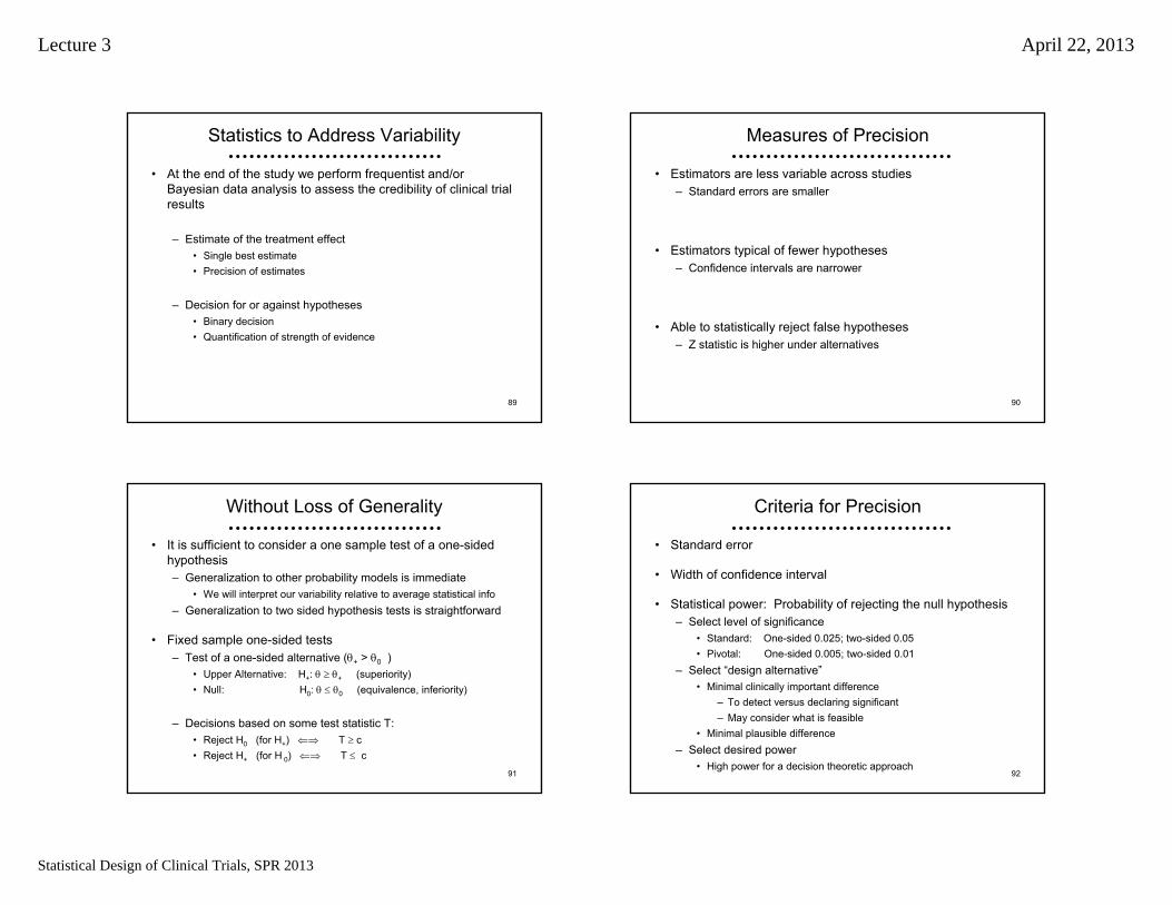
Statistics to Address Variability
• At the end of the study we perform frequentist and/or Bayesian data analysis to assess the credibility of clinical trial results
– Estimate of the treatment effect• Single best estimate• Precision of estimates
– Decision for or against hypotheses• Binary decision• Quantification of strength of evidence
90
Measures of Precision
• Estimators are less variable across studies– Standard errors are smaller
• Estimators typical of fewer hypotheses– Confidence intervals are narrower
• Able to statistically reject false hypotheses– Z statistic is higher under alternatives
91
Without Loss of Generality
• It is sufficient to consider a one sample test of a one-sided hypothesis– Generalization to other probability models is immediate
• We will interpret our variability relative to average statistical info– Generalization to two sided hypothesis tests is straightforward
• Fixed sample one-sided tests– Test of a one-sided alternative (+ > 0 )
• Upper Alternative: H+: + (superiority) • Null: H0: 0 (equivalence, inferiority)
– Decisions based on some test statistic T:• Reject H0 (for H+) T c • Reject H+ (for H 0) T c
92
Criteria for Precision
• Standard error
• Width of confidence interval
• Statistical power: Probability of rejecting the null hypothesis– Select level of significance
• Standard: One-sided 0.025; two-sided 0.05• Pivotal: One-sided 0.005; two-sided 0.01
– Select “design alternative”• Minimal clinically important difference
– To detect versus declaring significant– May consider what is feasible
• Minimal plausible difference– Select desired power
• High power for a decision theoretic approach

Lecture 3 April 22, 2013
Statistical Design of Clinical Trials, SPR 2013
93
Sample Size Determination
• Based on sampling plan, statistical analysis plan, and estimates of variability, compute
– Sample size that discriminates hypotheses with desired power,
OR
– Hypothesis that is discriminated from null with desired power when sample size is as specified, or
OR
– Power to detect the specific alternative when sample size is as specified
94
Sample Size Computation
) : testsample (Fixed
:units sampling Required
unit sampling 1 within y Variabilit ealternativDesign
when cesignifican of Levelpower with detected :1)(n test level edStandardiz
2/1
201
2
1
0
zz
Vn
V
95
When Sample Size Constrained
• Often (usually?) logistical constraints impose a maximal sample size– Compute power to detect specified alternative
– Compute alternative detected with high power
nV
01
01such that Find Vn
96
Without Loss of Generality
• Our ultimate interest is in comparing– Fixed sample tests– Group sequential tests– Other adaptive strategies
• We will thus further restrict attention to a one-sample setting in which– V = 1– Test of a one-sided alternative (+ > 0 )
• Upper Alternative: H+: + = 3.92 (superiority) • Null: H0: 0 = 0 (equivalence, inferiority)

Lecture 3 April 22, 2013
Statistical Design of Clinical Trials, SPR 2013
97
Fixed Sample Test
• Sample size N = 1 provides– Type 1 error of 0.025– Power of 0.975 to detect the alternative of 3.92– At the final analysis, an observed estimate (or Z statistic) of 1.96
will be statistically significant
• Power and sample size table
1.000.9753.92
1.000.9003.24
1.000.8002.80
1.000.5001.96
1.000.0250.00
Avg NPowerTrue Effect
98
Group Sequential Approach
• Perform analyses when sample sizes N1. . . NJ– Can be randomly determined if independent of effect
• At each analysis choose stopping boundaries– aj < bj < cj < dj
– Often chosen according to some boundary shape function• O’Brien-Fleming, Pocock, Triangular, …
• Compute test statistic Tj= T(X1. . . XNj)– Stop if Tj < aj (extremely low)– Stop if bj < Tj < cj (approximate equivalence)– Stop if Tj > dj (extremely high)– Otherwise continue
99
Stopping Boundary Scales
• Boundary scales (1:1 transformations among these)– Z statistic– P value
• Fixed sample (so wrong)• Computed under sequential sampling rule (so correct)
– Error spending function– Estimates
• MLE (biased due to stopping rule)• Adjusted for stopping rule
– Conditional power• Computed under design alternative• Computed under current MLE
– Predictive power• Computed under flat prior (possibly improper)
100
Exploring Group Sequential Designs
• Candidate designs– J = 2 equal spaced analyses; O’Brien-Fleming efficacy boundary
• Do not increase sample size (so lose power)• Maintain power under alternative (so inflate maximal sample size)
– J = 2 equal spaced analyses; OBF efficacy, futility boundaries• Do not increase sample size (so lose power)• Maintain power under alternative (so inflate maximal sample size)
– J = 2 equal spaced analyses; OBF efficacy, more efficient futility • Do not increase sample size (so lose power)• Maintain power under alternative (so inflate maximal sample size)
– J = 4 equal spaced analyses; OBF efficacy, more efficient futlility• Do not increase sample size (so lose power)• Maintain power under alternative (so inflate maximal sample size)
– J = 2 optimally spaced analyses; optimal symmetric boundaries• Maintain power under alternative (inflate NJ, but optimize ASN)

Lecture 3 April 22, 2013
Statistical Design of Clinical Trials, SPR 2013
101
Exploring Group Sequential Designs
• Examining operating characteristics– Stopping boundaries
• Z scale• Conditional power under hypothesized effects• Conditional power under current MLE• Predictive power under flat prior
– Estimates and inference• MLE (Bias adjusted estimates suppressed for space)• 95% CI properly adjusted for stopping rule• P value properly adjusted for stopping rule
– Power at specified alternatives– Sample size distribution (as function of true effect)
• Maximal sample size• Average sample size
102
O’Brien-Fleming Efficacy: J = 2
• Introduce two evenly spaced analyses– Type 1 error of 0.025
• Stopping boundary table
EfficacyFutilityInfoFrac PPflatCPestCPnullZPPflatCPestCPaltZ
------1.977------1.9771.0
0.9760.9970.5002.796--------0.5
103
O’Brien-Fleming Efficacy: J = 2, N = 1
• Introduce two evenly spaced analyses– Maintain sample size NJ = 1
• Estimates and inference table
EfficacyFutilitySampSize P95% CIMLEP95% CIMLE
0.025(0.00, 3.93)1.9770.025(0.00, 3.93)1.9771.0
0.003(1.16, 5.72)3.955------0.5
104
O’Brien-Fleming Efficacy: J = 2, N = 1
• Introduce two evenly spaced analyses– Maintain sample size NJ = 1
• Power and sample size table
0.7550.9743.92
0.8470.8983.24
0.8960.7972.80
0.9600.4961.96
0.9990.0250.00
Avg NPowerTrue Effect

Lecture 3 April 22, 2013
Statistical Design of Clinical Trials, SPR 2013
105
O’Brien-Fleming Efficacy: J = 2, Power
• Introduce two evenly spaced analyses– Maintain power 0.975 at alternative 3.92
• Estimates and inference table
EfficacyFutilitySampSize P95% CIMLEP95% CIMLE
0.025(0.00, 3.92)1.9770.025(0.00, 3.92)1.9771.01
0.003(1.16, 5.70)3.943------0.50
106
O’Brien-Fleming Efficacy: J = 2, Power
• Introduce two evenly spaced analyses– Maintain power 0.975 at alternative 3.92
• Power and sample size table
0.7580.9753.92
0.8510.9003.24
0.9010.7992.80
0.9660.4991.96
1.0050.0250.00
Avg NPowerTrue Effect
107
Take Home Messages 1
• Introduction of a very conservative efficacy boundary– Minimal effect on power even if do not increase max N– Minimal increase in max N needed to maintain power
• Ease and importance of evaluating a stopping rule– Even before we start the study, we can consider
• Thresholds for early stopping in terms of estimated effects• Inference corresponding to stopping points• Conditional and predictive power under various hypotheses
– We can judge a stopping rule by comparing it to a fixed sample test and look at the tradeoffs between
• Increase in maximal sample size• Decrease in average sample size• Changes in unconditional power
108
O’Brien-Fleming Symmetric: J = 2
• Introduce two evenly spaced analyses– Type 1 error of 0.025
• Stopping boundary table
EfficacyFutilityInfoFrac PPflatCPestCPnullZPPflatCPestCPaltZ
------1.977------1.9771.0
0.9760.9970.5002.7960.0240.0030.5000.0000.5

Lecture 3 April 22, 2013
Statistical Design of Clinical Trials, SPR 2013
109
O’Brien-Fleming Symmetric: J = 2, N = 1
• Introduce two evenly spaced analyses– Maintain sample size NJ = 1
• Estimates and inference table
EfficacyFutilitySampSize P95% CIMLEP95% CIMLE
0.025(0.00, 3.94)1.9730.025(0.00, 3.94)1.9731.0
0.003(1.15, 5.71)3.9450.375(-1.76, 2.80)0.0000.5
110
O’Brien-Fleming Symmetric: J = 2, N = 1
• Introduce two evenly spaced analyses– Maintain sample size NJ = 1
• Power and sample size table
0.7520.9743.92
0.8400.8973.24
0.8830.7952.80
0.9190.4951.96
0.7490.0250.00
Avg NPowerTrue Effect
111
O’Brien-Fleming Symmetric: J = 2, Power
• Introduce two evenly spaced analyses– Maintain power 0.975 at alternative 3.92
• Estimates and inference table
EfficacyFutilitySampSize P95% CIMLEP95% CIMLE
0.025(0.00, 3.92)1.9600.025(0.00, 3.92)1.9601.01
0.003(1.14, 5.67)3.9200.375(-1.75, 2.78)0.000.51
112
O’Brien-Fleming Symmetric: J = 2, Power
• Introduce two evenly spaced analyses– Maintain power 0.975 at alternative 3.92
• Power and sample size table
0.7580.9753.92
0.8480.9003.24
0.8930.8002.80
0.9300.5001.96
0.7580.0250.00
Avg NPowerTrue Effect

Lecture 3 April 22, 2013
Statistical Design of Clinical Trials, SPR 2013
113
Take Home Messages 2
• Introduction of a very conservative futility boundary– Again, minimal effects on power and/or max N– Dramatic improvement in ASN under the null– Conditional and predictive power thresholds are surprising
• CPalt = 0.50 for the extremely conservative OBF boundary– But the CI has already eliminated 3.92 with high confidence
• CPest = 0.003 and PPflat = 0.024 are both very low thresholds
114
O’Brien-Fleming & Futility: J = 2
• Introduce two evenly spaced analyses– Type 1 error of 0.025
• Stopping boundary table
EfficacyFutilityInfoFrac PPflatCPestCPnullZPPflatCPestCPaltZ
------1.963------1.9631.0
0.9750.9970.5002.7760.0680.0170.6440.3310.5
115
O’Brien-Fleming & Futility: J = 2, N = 1
• Introduce four evenly spaced analyses– Maintain sample size NJ = 1
• Estimates and inference table
EfficacyFutilitySampSize P95% CIMLEP95% CIMLE
0.025(0.00, 3.98)1.9630.025(0.00, 3.98)1.9631.0
0.003(1.13, 5.69)3.9250.228(-1.30, 3.27)0.4680.5
116
O’Brien-Fleming & Futility: J = 2, N = 1
• Introduce two evenly spaced analyses– Maintain sample size NJ = 1
• Power and sample size table
0.7470.9723.92
0.8300.8933.24
0.8690.7912.80
0.8860.4921.96
0.6840.0250.00
Avg NPowerTrue Effect

Lecture 3 April 22, 2013
Statistical Design of Clinical Trials, SPR 2013
117
O’Brien-Fleming & Futility: J = 2, Power
• Introduce two evenly spaced analyses– Maintain power 0.975 at alternative 3.92
• Estimates and inference table
EfficacyFutilitySampSize P95% CIMLEP95% CIMLE
0.025(0.00, 3.92)1.9340.025(0.00, 3.92)1.9341.03
0.003(1.11, 5.61)3.8670.228(-1.28, 3.22)0.4610.52
118
O’Brien-Fleming & Futility: J = 2, Power
• Introduce two evenly spaced analyses– Maintain power 0.975 at alternative 3.92
• Power and sample size table
0.7620.9753.92
0.8500.9013.24
0.8920.8032.80
0.9140.5041.96
0.7050.0250.00
Avg NPowerTrue Effect
119
Take Home Messages 3
• More aggressive futility boundary better addresses ethical issues associated with ineffective drugs– I often find that sponsors are willing to accept this futility bound
without increasing the sample size– But the minimal increase in maximal sample size would seem
more appropriate to me
120
O’Brien-Fleming & Futility: J = 4
• Introduce four evenly spaced analyses– Type 1 error of 0.025
• Stopping boundary table
------1.988------1.9881.00
0.8740.9070.5002.2950.1770.1420.5921.2580.75
EfficacyFutilityInfoFrac PPflatCPestCPnullZPPflatCPestCPaltZ
0.9770.9970.5002.8110.0630.0150.6480.3210.50
0.9990.9990.5003.9760.0080.0000.719-1.1080.25

Lecture 3 April 22, 2013
Statistical Design of Clinical Trials, SPR 2013
121
O’Brien-Fleming & Futility: J = 4, N = 1
• Introduce four evenly spaced analyses– Maintain sample size NJ = 1
• Estimates and inference table
0.025(0.00, 4.06)1.9880.025(0.00, 4.06)1.9881.00
0.013(0.30, 4.48)2.6500.053(-0.36, 3.85)1.4520.75
EfficacyFutilitySampSize P95% CIMLEP95% CIMLE
0.003(1.14, 6.04)3.9760.263(-1.60, 3.31)0.4540.50
0.000(4.00, 10.5)7.9510.846(-4.71, 1.74)-2.2160.25
122
O’Brien-Fleming & Futility: J = 4, N = 1
• Introduce four evenly spaced analyses– Maintain sample size NJ = 1
• Power and sample size table
0.6500.9663.92
0.7230.8823.24
0.7610.7762.80
0.7830.4781.96
0.5800.0250.00
Avg NPowerTrue Effect
123
O’Brien-Fleming & Futility: J = 4, Power
• Introduce four evenly spaced analyses– Maintain power 0.975 at alternative 3.92
• Estimates and inference table
0.025(0.00, 3.92)1.9200.025(0.00, 3.92)1.9201.07
0.013(0.29, 4.33)2.5610.053(-0.34, 3.72)1.4030.80
EfficacyFutilitySampSize P95% CIMLEP95% CIMLE
0.003(1.10, 5.84)3.8410.263(-1.55, 3.20)0.4390.54
0.000(3.86, 10.1)7.6820.846(-4.55, 1.68)-2.1410.27
124
O’Brien-Fleming & Futility: J = 4, Power
• Introduce four evenly spaced analyses– Maintain power 0.975 at alternative 3.92
• Power and sample size table
0.6800.9753.92
0.7620.9023.24
0.8080.8032.80
0.8400.5041.96
0.6220.0250.00
Avg NPowerTrue Effect

Lecture 3 April 22, 2013
Statistical Design of Clinical Trials, SPR 2013
125
Take Home Messages 4
• Effect of adding more analyses– Greater loss of power if maximal sample size not increased– Greater increase in maximal sample size if power maintained– But, improvement in average efficiency
• Can also use this example for guidance in how to judge thresholds for conditional and predictive power– The same threshold should not be used at all analyses– It is not, however, clear what threshold should be used
• I look at tradeoffs between average efficiency and power– We can look at optimal (on average) designs for more guidance
126
Efficient: J = 2
• Introduce two optimally spaced analyses to minimize ASN– Type 1 error of 0.025
• Stopping boundary table
EfficacyFutilityInfoFrac PPflatCPestCPnullZPPflatCPestCPaltZ
------2.129------2.1291.00
0.8590.9510.1822.7760.1410.0490.8180.5730.43
127
Efficient: J = 2, Power
• Introduce two optimally spaced analyses– Maintain power 0.975 at alternative 3.92
• Estimates and inference table
EfficacyFutilitySampSize P95% CIMLEP95% CIMLE
0.025(0.00, 3.92)1.9600.025(0.00, 3.92)1.9601.18
0.014(0.34, 4.74)3.1120.129(-0.82, 3.58)0.8080.50
128
Efficient: J = 2, Power
• Introduce two optimally spaced analyses– Maintain power 0.975 at alternative 3.92
• Power and sample size table
0.6850.9753.92
0.7880.9043.24
0.8470.8052.80
0.9000.5001.96
0.6850.0250.00
Avg NPowerTrue Effect

Lecture 3 April 22, 2013
Statistical Design of Clinical Trials, SPR 2013
129
Take Home Messages 5
• Optimal spacing of analyses not quite equal information
• Optimal early conservatism close to a Pocock design– In unified family, OBF has P=1, Pocock has P= 0.5– Optimal P= .54
• With two analyses, increase maximal N by 18% over fixed sample– ASN decreases by about one third
• Again, the thresholds to use for conditional or predictive power are not at all clear
• Search for best designs should include many candidates– Examine many operating characteristics
130
Spectrum of Boundary Shapes
• All of the rules depicted have the same type I error and power to detect the design alternative
131
Efficiency / Unconditional Power
• Tradeoffs between early stopping and loss of power
Boundaries Loss of Power Avg Sample Size
132
Delayed Measurement of Outcome
• Longitudinal studies– Measurement might be 6 months – 2 years after randomization– Interim analyses on variable lengths of follow-up
• Use of partial data can improve efficiency (Kittelson, et al.)
• Time to event studies– Statistical information proportional to number of events– Calendar time requirements depend on number accrued and
length of follow-up
• In either case: Interim analyses may occur after accrual completed
• Group ethics of identifying beneficial treatments faster• Savings in calendar time costs, rather than per patient costs

Lecture 3 April 22, 2013
Statistical Design of Clinical Trials, SPR 2013
Evaluation of Designs
134
Evaluation of Designs
• Process of choosing a trial design– Define candidate design
• Usually constrain two operating characteristics– Type I error, power at design alternative– Type I error, maximal sample size
– Evaluate other operating characteristics• Different criteria of interest to different investigators
– Modify design– Iterate
135
Collaboration of Disciplines
IssuesCollaboratorsDiscipline
Collection of data Study burdenData integrity
Study coordinatorsData managementOperational
Estimates of treatment effectPrecision of estimates
SafetyEfficacy
Cost effectivenessCost of trial / ProfitabilityMarketing appeal
Individual ethicsGroup ethics
Efficacy of treatmentAdverse experiences
Hypothesis generationMechanismsClinical benefit
BiostatisticiansStatistical
RegulatorsGovernmental
Health servicesSponsor managementSponsor marketers
Economic
EthicistsEthical
Experts in disease / treatmentExperts in complicationsClinical
EpidemiologistsBasic ScientistsClinical Scientists
Scientific
136
Which Operating Characteristics
• The same regardless of the type of stopping rule – Frequentist power curve
• Type I error (null) and power (design alternative)– Sample size requirements
• Maximum, average, median, other quantiles• Stopping probabilities
– Inference at study termination (at each boundary)• Frequentist or Bayesian (under spectrum of priors)
– (Futility measures• Conditional power, predictive power)

Lecture 3 April 22, 2013
Statistical Design of Clinical Trials, SPR 2013
137
At Design Stage
• In particular, at design stage we can know – Conditions under which trial will continue at each analysis
• Estimates– (Range of estimates leading to continuation)
• Inference– (Credibility of results if trial is stopped)
• Conditional and predictive power
– Tradeoffs between early stopping and loss in unconditional power
138
Operating Characteristics
• For any stopping rule, however, we can compute the correct sampling distribution with specialized software– From the computed sampling distributions we then compute
• Bias adjusted estimates• Correct (adjusted) confidence intervals• Correct (adjusted) P values
– Candidate designs are then compared with respect to their operating characteristics
139
Evaluation: Sample Size
• Number of subjects is a random variable– Quantify summary measures of sample size distribution as a
function of treatment effect• maximum (feasibility of accrual) • mean (Average Sample N- ASN) • median, quartiles
– Stopping probabilities• Probability of stopping at each analysis as a function of treatment
effect• Probability of each decision at each analysis
(Sponsor)(Sponsor, DMC)
(Sponsor)
140
Sample Size
• What is the maximal sample size required?– Planning for trial costs– Regulatory requirements for minimal N treated
• What is the average sample size required?– Hopefully low when treatment does not work or is harmful– Acceptable to be high when uncertainty of benefit remains– Hopefully low when treatment is markedly effective
• (But must consider burden of proof)

Lecture 3 April 22, 2013
Statistical Design of Clinical Trials, SPR 2013
141
ASN Curve
• Expected sample size as function of true effect
142
Evaluation: Power Curve
• Probability of rejecting null for arbitrary alternatives– Level of significance (power under null)– Power for specified alternative
– Alternative rejected by design • Alternative for which study has high power
– Interpretation of negative studies
(Scientists)
(Regulatory)
143
Evaluation: Boundaries
• Decision boundary at each analysis: Value of test statistic leading to early stopping– On the scale of estimated treatment effect
• Inform DMC of precision• Assess ethics
– May have prior belief of unacceptable levels• Assess clinical importance
– On the Z or fixed sample P value scales
(DMC)
(Marketing)
(DMC, Statisticians)
(Often asked for, but of
questionable relevance)
144
Evaluation: Inference
• Inference on the boundary at each analysis– Frequentist
• Adjusted point estimates• Adjusted confidence intervals• Adjusted P values
– Bayesian• Posterior mean of parameter distribution• Credible intervals• Posterior probability of hypotheses• Sensitivity to prior distributions
(Scientists,Statisticians, Regulatory)
(Scientists,Statisticians, Regulatory)

Lecture 3 April 22, 2013
Statistical Design of Clinical Trials, SPR 2013
145
Evaluation: Futility
• Consider the probability that a different decision would result if trial continued– Compare unconditional power to fixed sample test with same
sample size
– Conditional power• Assume specific hypotheses• Assume current best estimate
– Predictive power• Assume Bayesian prior distribution
(Scientists,Sponsor)
(Often asked for, but of
questionable relevance)
146
Efficiency / Unconditional Power
• Tradeoffs between early stopping and loss of power
• Boundaries Loss of Power Avg Sample Size
147
Evaluation: Marketable Results
• Probability of obtaining estimates of treatment effect with clinical or marketing appeal– Modified power curve
• Unconditional• Conditional at each analysis
– Predictive probabilities at each analysis
(Marketing,Clinicians)
Group Sequential Stopping Rules

Lecture 3 April 22, 2013
Statistical Design of Clinical Trials, SPR 2013
149
Stopping Rules
• Basic Strategy– Find stopping boundaries at each analysis such that desired
operating characteristics (e.g., type I and type II statistical errors) are attained
• Issues– Conditions under which the trial might be stopped early– When to perform analyses– Test statistic to use– Relative position of boundaries at successive analyses– Desired operating characteristics
150
Boundary Scales
• Stopping boundaries can be defined on a wide variety of scales – Sum of observations– Point estimate of treatment effect– Normalized (Z) statistic– Fixed sample P value– Error spending function– Conditional probability– Predictive probability– Bayesian posterior probability
151
Boundary Shape Function
• Boundary shape functions– j measures the proportion of information accrued at the j-th
analysis• often j = Nj / NJ
– Boundary shape function f(j) is a monotonic function used to relate the dependence of boundaries at successive analyses on the information accrued to the study at that analysis
152
Creating a RCT Design : Sequential
• seqDesign (nbr.analyses = 4, (default is 1)
sample.size = (1:4)/4*1700, (default spacing)
design.family = “X”, (default)
early.stopping = “both”, (default vs “null”, “alternative”)
P = c(1,1), (default corresponds to OBF)
A = c(0,0), (default)
R = c(0,0), (default)
minimum.constraint = , (default)
maximum.constraint = , (default)
exact.constraint = , (default)
(many others)
)

Lecture 3 April 22, 2013
Statistical Design of Clinical Trials, SPR 2013
153
Design Families
• RCTdesign allows specification of boundary shape functions on a variety of scales
• MLE (can also be specified on partial sum, Z) : – Unified family (Kittelson & Emerson, 1999)
• Error spending scale:– Power family (Kim & DeMets, 1987)– Hwang, Shih, DeCani (1990)
• RCTdesign also allows “constrained boundaries” that explicitly provide the boundary at one or more analyses
154
Common Framework
• Each stopping boundary is parameterized by– Hypothesized treatment effect rejected– Error probability or power with which that hypothesis is rejected
155
Unified Design Family
• Stopping Boundaries for MLE Statistic– Each boundary rejects a hypothesized value with some error– Lower, upper type 1 error; lower, upper power
• In a two-sided test with four boundaries
– Estimates below aj = a - fa (j) reject a (usually null) with lower type 1 error αL
– Estimates above bj = b + fb (j) reject b (lower alternative) with lower type 2 error 1-βL
– Estimates below cj = c - fc (j) reject c (upper alternative) with upper type 2 error 1-βU
– Estimates less than dj = d + fd (j) reject d (usually null) with upper type 1 error αU 156
Unified Design Family: Boundary Shape
• Parameterization of boundary shape functions
• Distinct parameters possible for each boundary
• Parameters A*, P*, R* typically chosen by user
• Critical value G* usually calculated from search to achieve desired error rates– Constraint that aJ = bJ and cJ = dJ
*** ])1([)( ** GAf Rj
Pjj

Lecture 3 April 22, 2013
Statistical Design of Clinical Trials, SPR 2013
157
Unified Design Family: Choosing P
• P 0:– Larger positive values of P make early stopping more difficult
(impossible when P infinite)– When A=R=0, 0.5 < P < 1 corresponds to power family
parameter () in Wang & Tsiatis (1987): P= 1 - – Reasonable range of values: 0 < P < 2.5– P=0 with A=R=0 possible for some (not all) boundaries, but not
particularly useful
158
Unified Design Family: P > 0, R = 0, A = 0
• Effect of varying P>0 (when A=0, R=0)– Higher P leads to early conservatism– P > 0 has infinite boundaries when N=0
159
Unified Design Family: Choosing P
• P < 0:– Must have R = 0 and (typically) A < 0– More negative values of P make early stopping more difficult
160
Unified Design Family: P < 0, R = 0, A = 0
• Effect of varying P<0 (when A=2, R=0)– More negative P leads to early conservatism– P < 0 has finite boundaries when N=0
Lecture 3 April 22, 2013
Statistical Design of Clinical Trials, SPR 2013
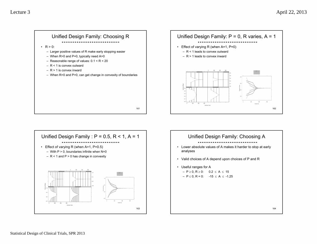
161
Unified Design Family: Choosing R
• R > 0:– Larger positive values of R make early stopping easier– When R>0 and P=0, typically need A>0– Reasonable range of values: 0.1 < R < 20– R < 1 is convex outward– R > 1 is convex inward – When R>0 and P>0, can get change in convexity of boundaries
162
Unified Design Family: P = 0, R varies, A = 1
• Effect of varying R (when A=1, P=0)– R < 1 leads to convex outward– R > 1 leads to convex inward
163
Unified Design Family : P = 0.5, R < 1, A = 1
• Effect of varying R (when A=1, P=0.5)– With P > 0, boundaries infinite when N=0– R < 1 and P > 0 has change in convexity
164
Unified Design Family: Choosing A
• Lower absolute values of A makes it harder to stop at early analyses
• Valid choices of A depend upon choices of P and R
• Useful ranges for A– P 0, R 0: 0.2 A 15– P 0, R = 0: -15 A -1.25

Lecture 3 April 22, 2013
Statistical Design of Clinical Trials, SPR 2013
165
Unified Design Family: P = 0, R = 1.2, A varies
• Effect of varying A (when P=0, R=1.2)– Values of A close to 0 make it harder to stop early– Higher absolute value of A -> flatter boundaries
166
Unified Design Family: Special Cases
• Parameterization of boundary shape function includes many previously described approaches
• Wang & Tsiatis Boundary Shape Functions:– A* = 0, R* = 0, P* > 0 – P* measures early conservatism
P* = 0.5 Pocock (1977)P* = 1.0 O’Brien-Fleming (1979)
– (P* = precludes early stopping)
• Triangular Test Boundary Shape Functions (Whitehead)– A* = 1, R* = 0, P* = 1
• Sequential Conditional Probability Ratio Test (Xiong):– R* = 0.5, P* = 0.5
167
Unified Design Family: Finding Designs
• Critical value G* usually calculated from iterative search to achieve desired error rates
• Starting estimates based on quantiles of standard normal
• Newtonian search (up to four dimensional)
• Constraint that aj = bj and cj = dj in standardized design
cRP
cdRP
ddcJJ
aRP
abRP
bbaJJ
Rj
Pjj
GAGAdc
GAGAba
GAf
ccdd
aabb
]01[]01[
]01[]01[
])1([)( *****
Specification of Designs
Error Spending Functions
Where am I going?The default family in RCTdesign is the Unified Family that includes a wide variety of previously described families.
RCTdesign also includes a number of designs defined on the error spending scale.
It is generally unimportant which scale is used for definition of a stopping rule, so long as they are fully evaluated
In my experience, people do not understand the scientific impact of particular error spending functions very well

Lecture 3 April 22, 2013
Statistical Design of Clinical Trials, SPR 2013
169
Error Spent at Each Analysis
• seqOC() returns stopping probabilities at each analysis
• When called under the null hypothesis, this is the error spent at each analysis
170
Error Spending Functions in RCTdesign
• No matter how a design is specified, RCTdesign returns the error spending function– “error.spend” component of a seqDesign object has the
cumulative proportion of error spent
– The efficacy boundary is the type 1 error spending function– The futility boundary is the type 2 error spending function for the
alternative used to define that boundary• (Need to fully understand the stopping boundaries)
171
Error Spending Families in RCTdesign
• seqDesign() argument design.family allows specification of error spending families
• design.family=“E”: extension of Kim & DeMets power family– If P < 0, then A = R = 0, G = 1– If P = 0, then A = -1, R < 0, G = 1
• design.family=“Hwang” uses Hwang, Shih, & DeCani family
*** ])1([)( ** GAf Rj
Pjj
)( :spentError ** jj f
0
01
11
1
)(*
P
Pe
ee
e
f
j
P
P
j
jj
172
Correspondences with Other Families
• Authors have described approximate correspondences to OBF and Pocock boundaries within unified family
• O’Brien – Fleming type error spending function– Lan and DeMets (1983)
– Kim and DeMets (1987) power family: P= -3– Hwang, Shih, and DeCani: P= -4 or -5
• Pocock type error spending function– Lan and DeMets (1983)
– Kim and DeMets (1987) power family: P= -1– Hwang, Shih, and DeCani: P= 1 (or P= 0?)
jj
zf *1
** 11)(
jj ef 11log)(*

Lecture 3 April 22, 2013
Statistical Design of Clinical Trials, SPR 2013
173
“O’Brien-Fleming” Design in Power Family
• I use P=-3.25 to approximate an OBF design– Others use P=-3
174
Comparison of Designs
• Overlay of O’Brien-Fleming design and approximation based on power family error spending function– plot(obf, obfE)
175
Relative Advantages
• Which is the best scale to view a stopping rule?– Maximum likelihood estimate– Z score / fixed sample P value– Error spending scale– Stochastic curtailment
• Conditional power• Predictive power
176
Current Relevance
• Many statisticians (unwisely?) focus on error spending scales, Z statistics, fixed sample P values when describing designs
• Some statisticians have (unwisely?) suggested the use of stochastic curtailment for– Defining prespecified sampling plans– Adaptive modification of sampling plans

Lecture 3 April 22, 2013
Statistical Design of Clinical Trials, SPR 2013
177
Z scale, Fixed Sample P value
• Interpretation of Z scale and fixed sample P value is difficult
178
Error Spending Functions
• My view: Poorly understood even by the researchers who advocate them
• There is no such thing as THE Pocock or O’Brien-Fleming error spending function– Depends on type I or type II error– Depends on number of analyses– Depends on spacing of analyses
179
OBF, Pocock Error Spending
180
Function of Alternative
• Error spending functions depend on the alternative used to compute them– The same design has many error spending functions
• JSM 2009: Session on early stopping for harm in a noninferiority trial– Attempts to use error spending function approach– How to calibrate with functions used for lack of benefit?

Lecture 3 April 22, 2013
Statistical Design of Clinical Trials, SPR 2013
181
Error Spent by Alternative
OBF Error Spending Functions by The
Cumulative Information
Pro
porti
on T
ype
I Err
or S
pent
0.0 0.2 0.4 0.6 0.8 1.0
0.0
0.2
0.4
0.6
0.8
1.0
0
0.025
0.05
0.075
Pocock Error Spending Functions by T
Cumulative Information
Pro
porti
on T
ype
I Erro
r Spe
nt
0.0 0.2 0.4 0.6 0.8 1.0
0.0
0.2
0.4
0.6
0.8
1.0
0
0.025
0.05
0.075
182
Stochastic Curtailment
• Stopping boundaries chosen based on predicting future data
• Probability of crossing final boundary– Frequentist: Conditional Power
• A Bayesian prior with all mass on a single hypothesis– Bayesian: Predictive Power
• Users are typically poor at guessing good thresholds– More on this later
Example
Series of RCT
Where am I going?The investigation of new treatments, preventive strategies, and diagnostic procedures typically progresses through several phases.
This example illustrates decisions that might be made between Phase II and Phase III
184
Example: ROC HS/D Shock Trial
• Resuscitation Outcomes Consortium– 11 Geographic sites serving ~ 20 million
• University based investigators – More than 250 EMS agencies
• Over 35,000 EMS providers: EMTs and paramedics
• Conduct definitive clinical trials in the resuscitation of pre-hospital cardiac arrest and severe traumatic injury– Treat patients 20-50 minutes on average before delivering them
to ED / hospital

Lecture 3 April 22, 2013
Statistical Design of Clinical Trials, SPR 2013
185
Hypertonic Resuscitation in Shock
• Hypotheses: Use of hypertonic fluids (instead of normal saline) in patients with hypovolemic shock– Osmotic action to maintain fluid in vascular space– Anti-inflammatory effect to minimize reperfusion injury
• Randomized, double blind clinical trial– Hypotensive subjects following trauma receive 250 ml bolus of
• 7.5% NaCl• 7.5% NaCl with dextran• Normal saline
– All other treatments per standard medical care
186
21 CFR 50.24
• Exception to informed consent for research in an emergency setting– Unmet need– Study effectiveness of a therapy with some preliminary evidence
of possible benefit– Consent impossible – Scientific question cannot be addressed in another setting– Patients in trial stand chance of benefit– Independent physicians attest to above– Community consultation / notification– As soon as possible notify subjects / next of kin of participation
and right to withdraw
187
Background: Phase II Study
• HS/D vs Lactate Ringers in shock from blunt trauma– Primary endpoint: ARDS free survival at 28 days
• Group sequential design– Planned maximal sample size: 400 patients (200 / arm)
• Interim results after 200 patients– 28 day ARDS-free survival : 54% with HSD, 64% with LRS– DMC recommendation: Stop for futility
• Trial results have excluded the hypothesized treatment effect
• Subgroup analysis– Suggestion of a benefit in the 20% needing massive transfusions
• 28 day ARDS-free survival: 13% with HSD, 0% with LRS– (Results must be quite unpromising in the other subgroup
Bulger, et al., Arch Surg 2008 143(2): 139 - 148.
188
ROC Phase III Study
• HS/D vs HS vs NS in shock from trauma– Primary endpoint: All cause survival at 28 days– Hypotheses: 69.2 % with HS/D or HS vs 64.6% with NS
• Eligibility criteria modified to try to exclude patients that do not require transfusion– Phase II study:
• SBP < 90 mmHg– Modification from exploratory analyses of Phase II data:
• SBP < 70 mmHg or• 70 mmHg < SBP < 90 mmHg and HR > 108

Lecture 3 April 22, 2013
Statistical Design of Clinical Trials, SPR 2013
189
Sample Size
• Fixed sample study:– Type I error 0.0125 due to multiple comparisons– 3,726 subjects regardless of observed treatment effect– Statistical significance if 4.1% improvement at end
• Group sequential monitoring:– No increase in maximal sample size– Therefore will have slight decrease in power depending on
stopping boundary that is chosen
190
Sample Size: Group Sequential Study
• Group sequential rule for efficacy: – “O’Brien-Fleming” rule known for “early-conservativism”– Maximal sample size 3,726
0.040 (0.005, 0.078); P = 0.01300.0422.2903,726Sixth
0.048 (0.010, 0.085); P = 0.00700.0522.5403,105Fifth
0.060 (0.019, 0.102); P = 0.00250.0652.8602,484Fourth
0.082 (0.035, 0.129); P = 0.00040.0883.3501,863Third
0.129 (0.070, 0.181); P < 0.00010.1344.1701,242Second
0.263 (0.183, 0.329); P < 0.00010.2726.000621First
Est (95% CI; One-sided P)Crude DiffZN
Accrue
Efficacy Boundary
191
Statistical License to Kill
• Initial evaluation of group sequential rule for futility– Considers noninferiority and superiority decisions
-0.2903,726Sixth
-0.7003,105Fifth
-1.2002,484Fourth
-1.8001,863Third
-2.8001,242Second
-4.000621First
ZN
Accrue
Futility Boundary
192
Statistical License to Kill
• Initial evaluation of group sequential rule for futility– Considers noninferiority and superiority decisions
0.050-0.2903,726Sixth
0.580.026-0.7003,105Fifth
0.610.010-1.2002,484Fourth
0.660.003-1.8001,863Third
0.680.000-2.8001,242Second
0.810.000-4.000621First
CP Noninf(hyp 4.8%)
Type II Error Spent (hyp 2.6%)Z
N Accrue
Futility Boundary

Lecture 3 April 22, 2013
Statistical Design of Clinical Trials, SPR 2013
193
Sample Size: Group Sequential Study
• Tentative group sequential rule for noninferiority: – DoD interested in lesser volume of fluid in battlefield if equivalent– Ultimately rejected by DMC due to lack of benefit for subjects
-0.003 (-0.041, 0.032); P = 0.5975-0.005-0.2903,726Sixth
-0.010 (-0.048, 0.028); P = 0.7090-0.014-0.7003,105Fifth
-0.022 (-0.064, 0.019); P = 0.8590-0.027-1.2002,484Fourth
-0.041 (-0.088, 0.006); P = 0.9581-0.047-1.8001,863Third
-0.084 (-0.137, -0.026); P = 0.9973-0.090-2.8001,242Second
-0.172 (-0.238, -0.092); P > 0.9999-0.181-4.000621First
Est (95% CI; One-sided P)Crude
DiffZN
Accrue
Futility Boundary
194
Sample Size: Group Sequential Study
• Group sequential rule for futility: – Based on rejecting the hypothesized treatment effect– Tradeoffs between average sample size and loss of power
0.043 (0.005, 0.080); P = 0.01250.0422.2763,726Sixth
0.038 (0.001, 0.078); P = 0.02090.0351.7403,105Fifth
0.030 (-0.011, 0.072); P = 0.07380.0251.1202,484Fourth
0.017 (-0.031, 0.063); P = 0.25910.0100.3721,863Third
-0.011 (-0.066, 0.045); P = 0.6684-0.019-0.6051,242Second
-0.088 (-0.154 -0.008); P = 0.9837-0.097-2.148621First
Est (95% CI; One-sided P)Crude
DiffZN
Accrue
Futility Boundary
195
Comparison of Average Sample Size
• Average number of subjects treated according to the true effect (benefit or harm) of the treatment
1,181 (.000)1,710 (.000)3,726 (.000)3,726 (.000)-0.06
1,473 (.000)2.374 (.000)3,726 (.000)3,726 (.000)-0.03
1,995 (.012)3,264 (.012)3,720 (.012)3,726 (.012)0.00
2,729 (.252)3,535 (.259)3,578 (.259)3,726 (.267)0.03
2,754 (.817)2,929 (.832)2,930 (.832)3,726 (.841)0.06
1,940 (.998) 1,968 (.999)1,968 (.999)3,726 (.999)0.10
Efficacy /Futility
Efficacy /Noninferiority
EfficacyOnly
FixedSample
TrueBenefit /
Harm
Average Sample Size (Power)
196
Benefit of Sequential Sampling
• Group sequential design can maintain type I error and power while greatly improving average sample size– To maintain power exactly, need slight increase in maximal N
• Improving average sample size increases number of beneficial treatments found by a consortium
• Advantage of group sequential over other adaptive strategies– Generally just as efficient– Better able to provide inference (“better understood” per FDA)

Lecture 3 April 22, 2013
Statistical Design of Clinical Trials, SPR 2013
197
Why Not “Scientific Adaptation”
• From Phase II to Phase III we modified patient population to try to remove nontransfused subjects– Subjects with low blood pressure due to fainting?– Subjects who died before treatment could be administered?
• Why not do this in the middle of a trial?– A priori: Need to confirm and provide inference for indication
• In hindsight: Phase III still showed increased mortality in thissubgroup that is identified post-randomization– Should we have modified treatment and/or eligibility?– More conservative approach in (at least) exception to informed
consent argues for careful evaluation of confusing results198
Final Comments
• In a large, expensive study, it is well worth our time to carefully examine the ways we can best protect– Patients on the study– Patients who might be on the study– Patients who will not be on the study, but will benefit from new
knowledge– Sponsor’s economic interests in cost of trial– Eventual benefit to health care – Eventual benefit to health care costs
• Adaptation to interim trial results introduces complications, but they can often be surmounted using methods that are currently well understood
199
Bottom Line
You better think (think)
about what you’re
trying to do…
-Aretha Franklin, “Think”
Case Study
A RCT of an Antibody to Endotoxin
in the Treatment of Gram Negative Sepsis

Lecture 3 April 22, 2013
Statistical Design of Clinical Trials, SPR 2013
201
The Enemy
“Let’s start at the very beginning, a very good place to start…”
- Maria von Trapp(as quoted by Rodgers and Hammerstein)
202
First
• Where do we want to be?
– Describe some innovative experiment?
– Find a use for some proprietary drug / biologic / device?• “Obtain a significant p value”
– Find a new treatment that improves health of some individuals• “Efficacy” seems to benefit some people somehow
– Find a new treatment that improves health of the population• “Effectiveness” requires proper use of a treatment that modifies an
important clinical endpoint
6
203
Treatment “Indication”
• Disease– Therapy: Putative cause vs signs / symptoms
• May involve method of diagnosis, response to therapies– Prevention / Diagnosis: Risk classification
• Population– Therapy: Restrict by risk of AEs or actual prior experience– Prevention / Diagnosis: Restrict by contraindications
• Treatment or treatment strategy– Formulation, administration, dose, frequency, duration, ancillary
therapies
• Outcome– Clinical vs surrogate; timeframe; method of measurement 204
Evidence Based Medicine: PICO
• Population (patient)– Disease– Restrictions due to concomitant disease, etc.
• Intervention– Treatment or treatment strategy
• Comparator– Other alternatives being considered
• Outcome– Clinical vs surrogate; timeframe; method of measurement

Lecture 3 April 22, 2013
Statistical Design of Clinical Trials, SPR 2013
205
Scientific Hypotheses: Background
• Critically ill patients often get overwhelming bacterial infection (sepsis), after which mortality is high
• Gram negative sepsis often characterized by production of endotoxin, which is thought to be the cause of much of the ill effects of gram negative sepsis
• Hypothesize that administering antibody to endotoxin may decrease morbidity and mortality
• Two previous randomized clinical trials showed slight benefit with suggestion of differences in benefit within subgroups
• No safety concerns
206
Indication
• Disease: Gram negative sepsis– Proven vs suspected– Gram stain, culture, abdominal injury
• Population: ICU patients
• Treatment– Single administration of antibody to endotoxin within 24 hours of
diagnosis of sepsis– Reductions in dose not applicable– Ancillary treatments unrestricted
• Outcome?
207
Clinical Outcomes
• Goals– Primary: Increase survival
• Long term (always best)• Short term (many other disease processes may intervene)
– Secondary: Decrease morbidity
• Relevant logistical considerations – Multicenter clinical trial
• Long term follow-up difficult in trauma centers• Data management is complicated
208
Candidate Clinical Outcomes
• Possible primary endpoints– Time to death
• Heavy early censoring due to constraints of trauma centers• May emphasize clinically meaningless short term improvements
– Mortality rate at fixed point in time• Allows choice of scientifically relevant time frame
– single administration; short half life• Allows choice of clinically relevant time frame
– avoid sensitivity to fleeting short term improvements– Time alive out of ICU during fixed period of time
• Incorporates morbidity endpoints• May be sensitive to clinically meaningless improvements depending
upon time frame chosen

Lecture 3 April 22, 2013
Statistical Design of Clinical Trials, SPR 2013
209
Trial Design Strategy
• Selection of clinical trial design is iterative, involving scientists, statisticians, management, and regulators
– Focus on measures with scientific meaning
– Search through extensive space of designs
– Compare designs with respect to variety of operating characteristics
210
Primary Endpoint: Statistical
• For a specific clinical endpoint, we still have to summarize itsdistribution
• Consider (in order or importance)– The most relevant summary measure of the distribution of the
primary endpoint• Based on a loss function?• Mean, median, geometric mean, …
– The summary measurement the treatment is most likely to affect– The summary measure that can be that can be assessed most
accurately and precisely
211
Statistical Design
• Steps– Defining the probability model
• Defining the comparison group, primary endpoint, analysis model– Defining the statistical hypotheses
• Null, alternative– Defining the statistical criteria for evidence
• Type I error, power– Determining the sample size
• At each analysis, and maximal sample size– Evaluating the operating characteristics– Planning for monitoring
• Updating stopping boundaries according to actual conditions– Plans for analysis and reporting results
• Inference adjusted for sequential sampling plan212
Chosen Endpoint / Study Structure
• Primary endpoint: 28 day all cause mortality
• Comparison group– Randomized, double blind, placebo controlled– 1:1 randomization
• Hypotheses– Treatment effect of 7% absolute increase in mortality
• On placebo: 30% 28 day mortality• On antibody: 23% 28 day mortality
• Burden of proof: Registrational trial– Type I error: one-sided 0.025– Statistical power: high

Lecture 3 April 22, 2013
Statistical Design of Clinical Trials, SPR 2013
213
Probability Models
• Common summary measures (contrasts) used in clinical trials– Means (difference)
• 1, 2, k arms; regression– Geometric means (lognormal medians) (ratio)
• 1, 2, k arms; regression– Proportions (difference)
• 1, 2 arms– Odds (ratio)
• 1, 2 arms; regression– Rates (ratio)
• 1, 2 arms; regression– Hazard (ratio)
• 2 arms
214
Creating a RCT Design : Model
• seqDesign (prob.model = “proportions”, (vs several others)
arms = 2, (default)
ratio = 1, (default)
variance = “alternative”, (default vs “null”,”intermediate”, number)
(many others)
)
215
Creating a RCT Design : Hypotheses
• seqDesign (null.hypothesis = 0.30,
alt.hypothesis = 0.23, (vs unspecified)
variance = “alternative”, (vs “null”,”intermediate” or number)
(many others)
)
216
Creating a RCT Design : Fixed Sample
• seqDesign (nbr.analyses = 1, (default)
test.type = “less”, (vs “greater”,”two.sided”)
size = 0.025, (default)
(many others)
)

Lecture 3 April 22, 2013
Statistical Design of Clinical Trials, SPR 2013
217
Creating a RCT Design : Statistical Task
• Provide two of alternative, power, sample size– seqDesign ( ) calculates the third
• Default values – Default power is from equal one-sided type 1 and 2 errors– If the alternative is specified, sample size merely indicates
spacing of analyses unless power calculation is explicitly specified
• seqDesign (alt.hypothesis = 0.23, (vs unspecified)
power = “calculate”, (vs a number, say, 0.90)
sample.size = 1700, (vs unspecified)
(many others)
) 218
Creating a RCT Design : Output
• seqDesign (display.scale = “X”, (default vs any boundary scale)
(many others)
)
219
Creating a RCT Design : GUI via Rcmdr (soon)
220
Evaluation of Fixed Sample Designs
• Clinical trial design is most often iterative– Specify an initial design– Evaluate operating characteristics– Modify the design– Iterate

Lecture 3 April 22, 2013
Statistical Design of Clinical Trials, SPR 2013
221
Fixed Sample Operating Characteristics
• Level of Significance (often pre-specified)
• Sample size requirements– Scientific / regulatory credibility; Feasibility
• Power Curve– Under null (type I error); design alternative
• Decision Boundary– Clinical significance
• Frequentist / Bayesian inference on the Boundary– Clinical significance of hypotheses discriminated– Sensitivity to Bayesian priors
222
Evaluation in RCTdesign
• Printing– Design: changeSeqScale (x, scale)
– Operating characteristics: seqOC (x, theta, power)
– Inference at boundary: seqInference (x)
– Everything: seqEvaluate (x, theta, power)
• Plotting– plot (x); seqPlotBoundary (x)
– seqPlotASN (x)
– seqPlotPower (x)
– seqPlotStopProb (x)
– seqPlotInference (x)
223
RCTdesign: Creation of Design
224
RCTdesign: evalGST

Lecture 3 April 22, 2013
Statistical Design of Clinical Trials, SPR 2013
225
Alternative Fixed Sample Designs
• Alternative sample sizes
• Sensitivity to assumptions about variability– Comparison of means, geometric means
• Need to estimate variability of observations– Comparison of proportions, odds, rates
• Need to estimate event rate– Comparison of hazards
• Need to estimate number of subjects and time required to observerequired number of events
226
What if Lower Event Rate?
227
What if Lower Event Rate?
228
Absolute vs Relative Differences
• When testing proportions, the alternative is routinely specifiedon one of two scales
• E.g.: When null = 0.30 and alternative = 0.23– Absolute difference: 0.23 – 0.30 = - 0.070 = - 7.0%– Relative difference: - 0.07 / 0.30 = - 0.233 = -23.3%
• Which to use?– Absolute difference relates to public health impact: effectiveness
• NNT = Number needed to treat to increase by 1 patient• In above example NNT = 1 / .07 = 14.3
– Relative difference might better assess efficacy• With a patient population “contaminated” by patients who survive
regardless, relative difference stays constant• E.g., with 50% contamination; 0.30 vs 0.23 0.15 vs 0.115

Lecture 3 April 22, 2013
Statistical Design of Clinical Trials, SPR 2013
229
Evaluation of Designs
• Process of choosing a trial design
– Define candidate design– Evaluate operating characteristics– Modify design– Iterate
230
Evaluation of Designs: Fixed Sample
• Operating characteristics for fixed sample studies
– Level of Significance (often pre-specified)– Sample size requirements– Power Curve– Decision Boundary– Frequentist inference on the Boundary– Bayesian posterior probabilities
231
Evaluation of Designs: Sequential
• Additional operating characteristics for group sequential studies
– Probability distribution for sample size– Stopping probabilities– Boundaries at each analysis– Frequentist inference at each analysis– Bayesian inference at each analysis– Futility measures at each analysis
232
Evaluation of Designs
• Sample size requirements – Number of subjects needed is a random variable
– Quantify summary measures of sample size distribution• maximum (feasibility of accrual)• mean (Average Sample N- ASN)• median, quartiles
– (Particularly consider tradeoffs between power and sample size distribution)

Lecture 3 April 22, 2013
Statistical Design of Clinical Trials, SPR 2013
233
Evaluation of Designs
• Stopping probabilities
– Consider probability of stopping at each analysis for arbitrary alternatives
– Consider probability of each decision (for null or alternative) at each analysis
234
Evaluation of Designs
• Power curve– Probability of rejecting null for arbitrary alternatives
• Power under null: level of significance• Power for specified alternative
– Alternative rejected by design• Alternative for which study has high power
– RCTdesign defines• Power curves for upper and lower boundaries• Alternatives having specified power for each boundary
235
Evaluation of Designs
• Decision boundary at each analysis– Value of test statistic leading to rejection of null
• Variety of boundary scales possible
– Often has meaning for applied researchers (especially on scale of estimated treatment effect)
• Estimated treatment effects may be viewed as unacceptable for ethical reasons based on prior notions
• Estimated treatment effect may be of little interest due to lack of clinical importance or futility of marketing
236
Evaluation of Designs
• Frequentist inference on the boundary at each analysis– Consider P values, confidence intervals when observation
corresponds to decision boundary at each analysis
– Ensure desirable precision for negative studies• Confidence interval identifies hypotheses not rejected by analysis• Have all scientifically meaningful hypotheses been rejected?

Lecture 3 April 22, 2013
Statistical Design of Clinical Trials, SPR 2013
237
Evaluation of Designs
• Bayesian posterior probabilities at each analysis
– Examine the degree to which the frequentist inference leads to sensible decisions under a range of prior distributions for the treatment effect
• Posterior probability of hypotheses
– Bayesian estimates of treatment effect• Median (mode) of posterior distribution• Credible interval (quantiles of posterior distribution
238
Evaluation of Designs
• Futility measures– Consider the probability that a different decision would result if
trial continued
– Can be based on particular hypotheses, current best estimate, orpredictive probabilities
– (Perhaps best measure of futility is whether the stopping rule has changed the power curve substantially)
239
O’Brien-Fleming Symmetric
240
O’Brien-Fleming Efficacy with Futility

Lecture 3 April 22, 2013
Statistical Design of Clinical Trials, SPR 2013
241
Plotting Stopping Boundaries
• plot() or seqPlotBoundary()– Arbitrary number of designs– By default, include fixed design with same power as first
specified design
• Axes– Y-axis: Critical values for stopping on arbitrary boundary scale
• MLE scale as default– X-axis: Statistical information
• Sample size (number of events for hazards probability models)
• Display of boundaries– Vertical lines are true stopping regions– Critical values connected to allow better visualization of
boundary shape 242
Display of Boundaries
• plot(obf, fut)
243
Plotting Power Functions
• seqPlotPower()– Arbitrary number of designs– By default, include fixed design with same maximal sample size
as first specified design
• Axes– Y-axis: Power or difference in power from reference design– X-axis: Treatment effect (θ)
• Interpretation based on probability model
244
Display of Power Curves
• seqPlotPower(obf, fut)

Lecture 3 April 22, 2013
Statistical Design of Clinical Trials, SPR 2013
245
Display of Power Curves (Reference)
• seqPlotPower(obf, fut, reference= T)
246
Plotting Sample Size Distribution
• seqPlotASN()– Arbitrary number of designs– Average sample N (ASN) and arbitrary quantiles
• Default is 75th percentile– By default, include fixed design with same power as first
specified design
• Axes– Y-axis: Statistical Information (average or quantile)– X-axis: Treatment effect (θ)
• Interpretation based on probability model
247
Display of ASN Curves
• seqPlotASN(obf, fut)
248
Plotting Stopping Probabities
• seqPlotStopProb()– Arbitrary number of designs
• By default, separate plots for each design• Different designs may have different sample sizes
– Essentially plots of error spending functions for each alternative
• Axes– Y-axis: Cumulative stopping probability– X-axis: Treatment effect (θ)
• Interpretation based on probability model– Contours labeled by analysis number
• May not correspond to same sample size– Color coding by decision corresponding to stopping rule

Lecture 3 April 22, 2013
Statistical Design of Clinical Trials, SPR 2013
249
Display of Stopping Probabilities
Comparison of Boundary Shape Function Families
Boundaries, ASN, Power, Stopping Probabilities
Where am I going?Families of group sequential boundary shape functions have been described on different boundary scales.
Generally a one parameter family of designs has enough flexibility to capture a range of suitable designs. In particular the Wang & Tsiatis family, Kim & DeMets error spending power family, and Hwang, Shih & DeCani error spending family behave quite similarly.
251
Probability of Continuing to Final Analysis
• Each of the three families of boundary shape functions can be viewed as a function of early conservatism
252
Similarity of Boundaries
• Grouping according to probability of continuing to final analysis
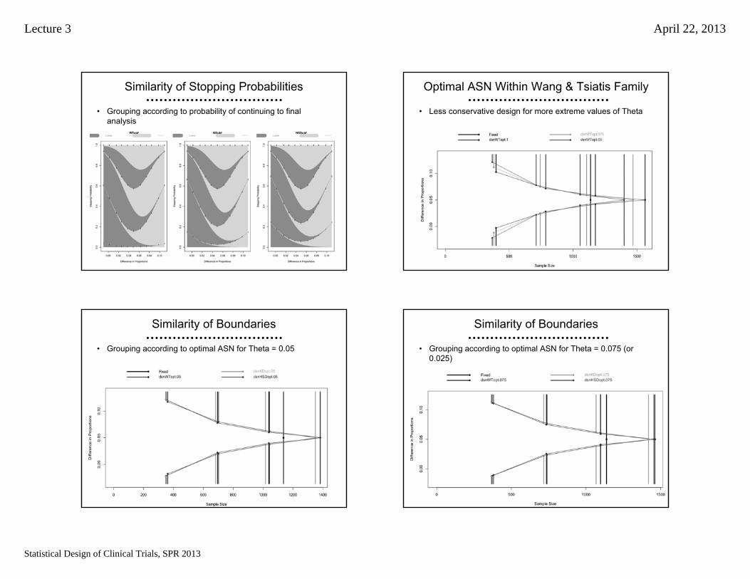
Lecture 3 April 22, 2013
Statistical Design of Clinical Trials, SPR 2013
253
Similarity of Stopping Probabilities
• Grouping according to probability of continuing to final analysis
254
Optimal ASN Within Wang & Tsiatis Family
• Less conservative design for more extreme values of Theta
255
Similarity of Boundaries
• Grouping according to optimal ASN for Theta = 0.05
256
Similarity of Boundaries
• Grouping according to optimal ASN for Theta = 0.075 (or 0.025)

Lecture 3 April 22, 2013
Statistical Design of Clinical Trials, SPR 2013
257
Similarity of Boundaries
• Grouping according to optimal ASN for Theta = 0.1 (or 0)
258
Similarity of Power Curves
• Grouping according to optimal ASN for Theta = 0.1 (or 0)
259
Similarity of ASN Curves
• Grouping according to optimal ASN for Theta = 0.1 (or 0)
260
Similarity of Stopping Probabilities
• Grouping according to optimal ASN for Theta = 0.1 (or 0)

Lecture 3 April 22, 2013
Statistical Design of Clinical Trials, SPR 2013
Stochastic Curtailment:“Futility” Boundary Scales
Conditional, Predictive Power
Where am I going?There is a 1:1 correspondence among the various boundary scales used to describe stopping boundaries. Hence it should not matter which scale is used to define boundaries.
However, I find that the stochastic curtailment scales are poorly understood.
262
Stochastic Curtailment
• Stopping boundaries chosen based on predicting future data
• Probability of crossing final boundary– Frequentist: Conditional Power
• A Bayesian prior with all mass on a single hypothesis– Bayesian: Predictive Power
263
But What If?
• It is common for people to ask about the possibility of a reversed decision– But suppose we did not stop for futility. What would be the
probability of getting a significant result if we continued to the maximal sample size
• This is easily computed conditional on the observed results IF we know the true treatment effect– Conditional power: Assume a particular effect– Predictive power: Use a Bayesian prior distribution
264
Stochastic Curtailment
• Boundaries transformed to conditional or predictive power
• Key issue: Computations are based on assumptions about the true treatment effect
• Conditional power– “Design”: based on hypotheses– “Estimate”: based on current estimates
• Predictive power– “Prior assumptions”

Lecture 3 April 22, 2013
Statistical Design of Clinical Trials, SPR 2013
265
Conditional/Predictive Power
Futility (rejects -0.0866)Futility (rejects -0.0855)
O’Brien-Fleming Efficacy, P=0.8 FutilitySymmetric O’Brien-Fleming
0.1770.3120.1420.592-0.0310.1240.2410.0910.500-0.0281275
0.0630.2470.0150.648-0.0100.0230.1430.0020.5000.000850
0.0080.2220.0000.7190.0470.0000.0770.0000.5000.085425
0.1260.0770.0930.500-0.0570.1240.0770.0910.500-0.0571275
0.0230.0150.0020.500-0.0850.0230.0150.0020.500-0.085850
0.0000.0020.0000.500-0.1700.0000.0020.0000.500-0.171425
Efficacy (rejects 0.00)Efficacy (rejects 0.00)NoninfSponsorEstimateDesignMLENoninfSponsorEstimateDesignMLEN
Predictive PowerConditional PowerPredictive PowerConditional Power
266
So What?
• Why not use stochastic curtailment?
• What treatment effect should we presume?– Hypothesis rejected; current estimate?
• What threshold should be used for a “low” probability– Choice of thresholds poorly understood
• 10%, 20%, 50%, 80%?• How should it depend on sample size and treatment effect
• Inefficient designs result– Conditional and predictive power do not correspond directly to
unconditional power
267
Assumed Effect and Threshold
• Probability threshold should take into account the timing of theanalysis and the presumed treatment effect
• It is not uncommon for naïve users to condition on a treatment effect that has already been excluded
268
Predictive Power: Example 1
• Sepsis trial to detect difference in 28 day survival: – Null 0.00 vs Alt -0.07 (90% power)
• Futility boundary at first of 4 analyses– Futile if observed diff > 0.0473 (so wrong direction)– Inference at boundary
• Bias adjusted: 0.038 (95% CI -0.037 to 0.101)

Lecture 3 April 22, 2013
Statistical Design of Clinical Trials, SPR 2013
269
Predictive Power: Example 1
• MLE: 0.0473 Bias Adj: 0.038 (CI: -0.037, 0.101)
Presumed Predictive
True Effect Power
-0.086 71.9%
-0.070 43.2%
-0.037 10.3%
Spons prior 2.8%
Flat prior 0.8%
0.047 <0.005%
270
Predictive Power: Ex 2 (OBF)
• Sepsis trial to detect difference in 28 day survival: – Null 0.00 vs Alt -0.07 (90% power)
• Futility bounday at first of 4 analyses– Futile if observed diff > 0.0855 (so wrong direction)– Inference at boundary
• Bias adjusted: 0.077 (95% CI 0.000 to 0.139)
271
Predictive Power: Ex 2 (OBF)
• MLE: 0.0855 Bias Adj: -0.077 (CI: 0.000, 0.139)
Presumed Predictive
True Effect Power
-0.086 50.0%
-0.070 26.5%
0.000 .03%
Spons prior 0.3%
Flat prior 0.03%
0.085 <0.005%
272
Key Issues
• Very different probabilities based on assumptions about the true treatment effect
• Extremely conservative O’Brien-Fleming boundaries correspond to conditional power of 50% (!) under alternative rejected by the boundary
• Resolution of apparent paradox: if the alternative were true, there is less than .003 probability of stopping for futility at the first analysis

Lecture 3 April 22, 2013
Statistical Design of Clinical Trials, SPR 2013
273
Stopping Probs for = -0.07
Group Sequential test
Efficacy Futility
N= 425 0.009 < - 0.170 > 0.047 0.003
N= 850 0.298 < - 0.085 > - 0.010 0.022
N= 1275 0.401 < - 0.057 > - 0.031 0.039
N= 1700 0.179 < - 0.042 > - 0.042 0.048
Total 0.888 0.112
274
Apples with Apples
• Can compare a group sequential rule to a fixed sample test providing– Same maximal sample size (N= 1700)– Same (worst case) average sample size (N= 1336)– Same power under the alternative (N= 1598)
• Consider probability of “discordant decisions”– Conditional probability (conditional power)– Unconditional probability (power)
275
Comparable Power for = -0.07
• Boundaries based on MLE
Group Sequential testEfficacy Futility
N= 425 < - 0.170 > 0.047N= 850 < - 0.085 > - 0.010N= 1275 < - 0.057 > - 0.031N= 1700 < - 0.042 > - 0.042
Fixed Sample Test
N= 1598 < - 0.043 > - 0.043
276
Stopping Probs for = -0.07
Group Sequential testEfficacy Futility
N= 425 0.009 < - 0.170 > 0.047 0.003N= 850 0.298 < - 0.085 > - 0.010 0.022N= 1275 0.401 < - 0.057 > - 0.031 0.039N= 1700 0.179 < - 0.042 > - 0.042 0.048
Total 0.888 0.112
Fixed Sample Test
N= 1598 0.888 < - 0.043 > - 0.043 0.112

Lecture 3 April 22, 2013
Statistical Design of Clinical Trials, SPR 2013
277
Cond Prob of Discordance
Group Sequential testEfficacy Futility
N= 425 0.002 < - 0.170 > 0.047 0.348N= 850 0.003 < - 0.085 > - 0.010 0.263N= 1275 0.009 < - 0.057 > - 0.031 0.172N= 1700 0.094 < - 0.042 > - 0.042 0.182
Total 0.024 0.197
Fixed Sample Test
N= 1598 < - 0.043 > - 0.043
278
Uncond Prob of Discordance
Group Sequential testEfficacy Futility
N= 425 0.009 < - 0.170 > 0.047 0.001N= 850 0.001 < - 0.085 > - 0.010 0.006N= 1275 0.004 < - 0.057 > - 0.031 0.007N= 1700 0.017 < - 0.042 > - 0.042 0.009
Total 0.022 0.022
Fixed Sample Test
N= 1598 < - 0.043 > - 0.043
279
Stopping Probs for = -0.07
Group Sequential testEfficacy Futility
N= 425 0.009 < - 0.170 > 0.047 0.003N= 850 0.298 < - 0.085 > - 0.010 0.022N= 1275 0.401 < - 0.057 > - 0.031 0.039N= 1700 0.179 < - 0.042 > - 0.042 0.048
Total 0.888 0.112
Fixed Sample Test
N= 1598 0.888 < - 0.043 > - 0.043 0.112
280
Cond/Uncond Comparison
Group Sequential testEfficacy Futility
Cond Uncond Cond UncondN= 425 0.002 0.000 0.348 0.001N= 850 0.003 0.001 0.263 0.006N= 1275 0.009 0.004 0.172 0.007N= 1700 0.094 0.017 0.182 0.009
Total 0.024 0.022 0.197 0.022
Lecture 3 April 22, 2013
Statistical Design of Clinical Trials, SPR 2013
281
Ordering of the Outcome Space
• Choosing a threshold based on conditional power can lead to nonsensical orderings based on unconditional power
• Decisions based on 35% conditional power may be more conservative than decisions based on 18% conditional power
• Can result in substantial inefficiency (loss of power)
282
Other Comparisons
• In the previous example, the fixed sample design had the same power as the GST
• If we instead compare a fixed sample test having same worst case ASN, the GST would have greater power
• If we compare a fixed sample test having same maximal N, the GST has less power
283
Further Comments
• Neither conditional power nor predictive power have good foundational motivation
• Frequentists should use Neyman-Pearson paradigm and consider optimal unconditional power across alternatives– And conditional/predictive power is not a good indicator in loss of
unconditional power
• Bayesians should use posterior distributions for decisions
Implementation for Monitoring

Lecture 3 April 22, 2013
Statistical Design of Clinical Trials, SPR 2013
285
Schedule of Analyses
• Design of clinical trial : Selection of stopping rule to providedesired operating characteristics– Type I error– Statistical power to detect design alternative– Efficiency– Bayesian properties– Futility considerations
286
Schedule of Analyses
• At time of study design : Sample size (power, alternative) calculations based on– Specifying a maximum of J analyses– Specifying sample sizes at which analyses will be performed
• During conduct of study: Number and timing of analyses may be different– Monitoring scheduled by calendar time– Slow (or fast) accrual– Estimation of available information at time of locking database– External causes– (should not be influenced by study results)
287
Impact of Altered Schedule
• Summary for Pocock boundary relationships
Analysis Times Alt Max N Bound======================== ==== ====== =====.25, .50, .75, 1.00 .500 345.23 .2500.40, .60, .80, 1.00 .500 329.91 .2500.40, .60, .80, 1.00 .489 345.23 .2444.20, .40, .60, .80, 1.00 .500 360.51 .2500.20, .40, .60, .80, 1.00 .511 345.23 .2555
288
Impact of Altered Schedule
• Summary for O’Brien-Fleming boundary relationships
Analysis Times Alt Max N Bound======================== ==== ====== =====.25, .50, .75, 1.00 .500 256.83 .2500.40, .60, .80, 1.00 .500 259.44 .2500.40, .60, .80, 1.00 .503 256.83 .2513.20, .40, .60, .80, 1.00 .500 259.45 .2500.20, .40, .60, .80, 1.00 .503 256.83 .2513

Lecture 3 April 22, 2013
Statistical Design of Clinical Trials, SPR 2013
289
Implementation
• Need methods that allow flexibility in determining number and timing of analyses
• Should maintain some (but not, in general, all) desired operating characteristics, e.g.:– Type I error– Type II error– Maximal sample size– Futility properties– Bayesian properties
290
Estimation of Statistical Information
• At time of study design: Sample size (power, alternative) calculations based on– Specifying statistical information available from each sampling
unit
• During conduct of study: Statistical information from a sampling unit may be different than originally estimated– Variance of measurements– Baseline event rates– (Altered sampling distribution for treatment levels)
291
Estimation of Statistical Information
• Effect of using incorrect estimates of statistical information at the design stage– Using the specified sample size, the design alternative will not
be detected with the desired power
– Using the specified sample size, the alternative detected with the desired power will not be the design alternative
– In order to detect the design alternative with the desired power, a different sample size is needed
292
Blinded Adaptive Sampling
• Modify sample size to account for estimated information (variance or baseline rates)
• No effect on type I error IF– Estimated information independent of estimate of treatment
effect• Proportional hazards,• Normal data, and/or• Carefully phrased alternatives
– And willing to use conditional inference• Carefully phrased alternatives

Lecture 3 April 22, 2013
Statistical Design of Clinical Trials, SPR 2013
293
Estimation of Statistical Information
• If maximal sample size is maintained, the study discriminates between null hypothesis and an alternative measured in units of statistical information
V
nVn2
01
21
201
21
)()(
294
Estimation of Statistical Information
• If statistical power is maintained, the study sample size is measured in units of statistical information
201
21
201
21
)()(
VnVn
295
Schedule of Analyses
• Use of constrained families is necessary because critical values are dependent upon exact schedule– In Unified Family, boundary at first analysis is affected by timing
of later analyses
– Compare boundary at first analysis when timing of second analysis differs:
• `a’ boundary: -0.0743 versus -0.0740• ‘d’ boundary: 0.5744 versus 0.5713
– Must constrain first boundaries at the levels actually used, andthen use parametric form for future analyses
296
Flexible Determination of Boundaries
• When implementing stopping rules, must be able to accommodate changes
• Previously described methods for implementing stopping rules– (Adhere exactly to monitoring plan)– (Approximations based on design parameters: Emerson and
Fleming, 1989)– Christmas tree approximation for triangular tests: Whitehead and
Stratton, 1983– Error spending functions: Lan and DeMets, 1983; Pampallona,
Tsiatis, and Kim, 1995– Constrained boundaries in unified design family: Emerson, 2000;
Burington and Emerson, 2003

Lecture 3 April 22, 2013
Statistical Design of Clinical Trials, SPR 2013
297
Common Features
• Stopping rule specified at design parameterizes the boundary for some statistic (boundary scale)
• At the first interim analysis, parametric form is used to compute the boundary for actual time on study
• At successive analyses, the boundaries are recomputed accounting for the exact boundaries used at previously conducted analyses
• Maximal sample size estimates may be updated
298
Constrained Boundaries Approach
• Use of constrained families in flexible implementation of stopping rules– At the first analysis, compute stopping boundary from parametric
family
– At successive analyses, use parametric family with constraints (on some scale) for the previously conducted interim analyses
– When the error spending scale is used, this is just the error spending approach of Lan & DeMets or Pampallona, Tsiatis, & Kim
299
Case Study: Summary of Study
• Target population– Patients in ICU with newly diagnosed gram negative sepsis
• Primary endpoint– 28 day mortality (binary)
• Summary measure (contrast)– Difference in probability of mortality within 28 days
• Test type– One-sided level .025 test of binomial proportions
• Baseline event rate and clinically relevant difference– Assumed to be 30%– 5% absolute difference in 28 day mortality 300
Case Study: Monitoring the Trial
• Maintaining operating characteristics– Depends upon statistical information
– In the binomial case, this is determined by the event rates
– If event rates are different from those assumed at design stage,need to choose whether to
• Re-estimate maximum sample size to maintain power• Maintain maximum sample size and re-compute power
– Re-compute these by using the POOLED event rate on observed data

Lecture 3 April 22, 2013
Statistical Design of Clinical Trials, SPR 2013
301
• Simulated example– Event rate in control arm is 0.35– Event rate in treatment arm is 0.25
• First interim analysis takes place after 400 patients observed (200 per arm)
Case Study: Simulated Monitoring
302
First Monitoring Analysis: Re-estimate N
303
First Monitoring Analysis
304
Second Monitoring Analysis

Lecture 3 April 22, 2013
Statistical Design of Clinical Trials, SPR 2013
305
Second Monitoring Analysis
Time to Event Endpoints
Estimating Subject Accrual
Where am I going?In time to event analyses, statistical information is roughly proportional to the number of events.
Additional consideration must be given to accrual of subjects.
307
Time to Event Endpoints
• RCTdesign allows specification of the “hazard” probability model for time to event data– Logrank statistic– Estimates of hazard ratio using Cox model
• “Sample size” computations return number of events primarily
• Additional accrual models are used to estimate– Number of subjects to accrue– Calendar time of interim analyses
308
Case Study: Stopping Rule
• Design of RCT to test a new drug for NSCLC– One-sided type 1 error: 0.025 for null of HR=1.0– Power: 90% to detect HR= 0.77– Four interim analyses with OBF efficacy, intermediate futility

Lecture 3 April 22, 2013
Statistical Design of Clinical Trials, SPR 2013
309
Specification of Accrual
• Need to observe 655 events
• Accrual pattern can be specified in a variety of ways– Accrual and additional follow-up time
• Calculates accrual rate– Accrual rate and study time
• Calculates accrual time
• Wide variety of distributions for– Accrual (uniform, beta, rates for each time period)– Loss to follow-up (exponential, Weibull, piecewise exponential)– Time to event (exponential, Weibull, piecewise exponential)
• Accrual parameters can be specified in seqDesign()310
Case Study: Accrual
• Need to observe 655 events
• Assume accrual over 3 years– Use uniform accrual
• Assume additional follow-up of 1 year– Total study time of 4 years
• Assume median survival of 3 years– Use exponential survival distribution
311
Case Study: Accrual
• tte <- update(tte, accrualTime= 3, studyTime= 4, eventQuantiles= 3)
312
Case Study: Accrual (months)
• tte <- update(tte, accrualTime= 36, studyTime= 48, eventQuantiles= 36)

Lecture 3 April 22, 2013
Statistical Design of Clinical Trials, SPR 2013
313
Case Study: Accrual Plots
• seqPlotPHNSubjects(tte)
314
Case Study: Accrual Plots
• seqPlotPHNSubjects(tte)
Response Adaptive Modificationsof an RCT Design
Overview of General Methods
Where am I going?Various authors have advocated the use of unblinded interim estimates of the treatment effect to modify a broad spectrum of RCT design parameters.
In this section of this course, I review the most commonly espoused statistical methods that would be used to maintain an experimentwise type I error.
316
Blinded Adaptive Sampling
• Modify sample size to account for estimated information (variance or baseline rates)
• No effect on type I error IF– Estimated information independent of estimate of treatment
effect• Proportional hazards,• Normal data, and/or• Carefully phrased alternatives
– And willing to use conditional inference• Carefully phrased alternatives

Lecture 3 April 22, 2013
Statistical Design of Clinical Trials, SPR 2013
317
Estimation of Statistical Information
• If maximal sample size is maintained, the study discriminates between null hypothesis and an alternative measured in units of statistical information
V
nVn2
01
21
201
21
)()(
318
Estimation of Statistical Information
• If statistical power is maintained, the study sample size is measured in units of statistical information
201
21
201
21
)()(
VnVn
319
Adaptation to Gain Efficiency?
• Consider adaptation merely to repower study– “We observed a result that was not as good as we had
anticipated”
• All GST are within family of adaptive designs– Don’t we have to be at least as efficient?
• Issues– Unspecified adaptations– Comparing apples to apples
320
Two Stage Design
• Proschan & Hunsberger consider worst case
– At first stage, choose sample size of second stage• N2 = N2(Z1) to maximize type I error
– At second stage, reject if Z2 > a2

Lecture 3 April 22, 2013
Statistical Design of Clinical Trials, SPR 2013
321
Proschan & Hunsberger
• Worst case type I error of two stage design
• Can be more than two times the nominal– a2 = 1.96 gives type I error of 0.0616– (Compare to Bonferroni results)
,4
2/exp12)(
2)(2
ZZ
worstaa
322
Flexible Adaptive Designs
• Proschan and Hunsberger describe adaptations to maintain experimentwise type I error and increase conditional power– Must prespecify a conditional error function
– Often choose function from some specified test
– Find critical value to maintain type I error
323
Other Approaches
• Self-designing Trial (Fisher, 1998)– Combine arbitrary test statistics from sequential groups– Prespecify weighting of groups “just in time”
• Specified at immediately preceding analysis– Fisher’s test statistic is N(0,1) under the null hypothesis of no
treatment difference on any of the endpoints tested
• Combining P values (Bauer & Kohne, 1994)– Based on R.A. Fisher’s method
324
Incremental Statistics
• Statistic at the j-th analysis a weighted average of data accrued between analyses
.ˆ
ˆ
ˆ :incrementth on computed Statistics
*
1
**
1
*
***
1*
j
k
j
kk
jj
k
j
kk
j
kkk
kkk
N
ZNZ
N
N
PZk
NNN

Lecture 3 April 22, 2013
Statistical Design of Clinical Trials, SPR 2013
325
Conditional Distribution
.1,0~|
1,/
~|
,~|ˆ
0**
*0**
***
UH
NP
NVNNZ
NVNN
jj
j
jj
jjj
326
Protecting Type I Error
• LD Fisher’s variance spending method– Arbitrary hypotheses H0j:θj = θ0j
– Incremental test statistics Zj*
– Allow arbitrary weights Wj specified at stage j-1
• RA Fisher’s combination of P values (Bauer & Köhne)
j
kjj
J
kj
k
J
kk
j
PP
W
ZWZ
1
*
1
*
1
327
Unconditional Distribution
• Under the null– SDCT: Standard normal– Bauer & Kohne: Sum of exponentials
• Under the alternative– Unknown unless prespecified adaptations
.Pr|PrPr0
****
n
jjjj nNNzZzZ
328
Sufficiency Principle
• It is easily shown that a minimal sufficient statistic is (Z, N) at stopping
• All methods advocated for adaptive designs are thus not based on sufficient statistics

Lecture 3 April 22, 2013
Statistical Design of Clinical Trials, SPR 2013
Response Adaptive Modificationsof an RCT Design
Modification of the Maximal Sample Size
Where am I going?The majority of the statistical literature on adaptive clinical trial design is directed toward using interim estimates of the treatment effect to re-power a study.
In this section of the course I review the basis for those methods and demonstrate the settings in which such adaptive designs can improve substantially on more traditional methods.
330
Adaptive Sample Size Determination
• Design stage: – Choose an interim monitoring plan– Choose an adaptive rule for maximal sample size
• Conduct stage: – Recruit subjects, gather data in groups– After each group, analyze for DMC
• DMC recommends termination or continuation– After penultimate group, determine final N
• Analysis stage: – When study stops, analyze and report
331
Adaptive Sample Size Approach
• Perform analyses when sample sizes N1. . . NJ• N1. . . NJ-1 can be randomly determined indep of effect
• At each analysis choose stopping boundaries• aj < bj < cj < dj
• At N1. . . NJ-1 compute test statistic Tj= T(X1. . . XNj)• Stop if Tj < aj (extremely low)• Stop if bj < Tj < cj (approximate equivalence)• Stop if Tj > dj (extremely high)• Otherwise continue
– At NJ-1 determine NJ according to value of Tj
332
Operating Characteristics
• Given an adaptive rule that modifies the final sample size at the penultimate stage, this can be viewed as adaptively switching between two group sequential tests– Standard group sequential software can be used

Lecture 3 April 22, 2013
Statistical Design of Clinical Trials, SPR 2013
333
Apples with Apples
• Can adapting beat a GST with the same number of analyses?– Fixed sample design: N=1– Most efficient symmetric GST with two analyses
• N = 0.5, 1.18• ASN = 0.6854
– Most efficient adaptive design with two possible N• N = 0.5 and either 1.06 or 1.24• ASN = 0.6831 ( 0.34% more efficient)
– “Most efficient” adaptive design with four possible N• N = 0.5 and either 1.01, 1.10, 1.17, or 1.31• ASN = 0.6825 ( 0.42% more efficient)
334
Apples with Apples (continued)
• GST with more analyses?– Fixed sample design: N=1– Most efficient symmetric GST with two analyses
• N = 0.5, 1.18• ASN = 0.6854
– GST with same three analyses• N = 0.5,1.06 and 1.24• ASN = 0.6666 ( 2.80% more efficient)
– GST with same five analyses• N = 0.5, 1.01, 1.10, 1.17, or 1.31• ASN = 0.6576 ( 4.20% more efficient)
335
Prespecified Modification Rules
• Adaptive sampling plans exact a price in statistical efficiency
• Tsiatis & Mehta (2002); Jennison & Turnbull (2003)– A classic prespecified group sequential stopping rule can be
found that is more efficient than a given adaptive design
• Shi (2003, unpublished thesis)– Fisher’s test statistic in the self-designing trial provides markedly
less precise inference than that based on the MLE• To compute the sampling distribution of the latter, the sampling plan
must be known
336
Comments re Conditional Power
• Many authors propose adaptations based on conditional or predictive power
• Neither conditional power nor predictive power have good foundational motivation– Frequentists should use Neyman-Pearson paradigm and
consider optimal unconditional power across alternatives• And conditional/predictive power is not a good indicator in loss of
unconditional power– Bayesians should use posterior distributions for decisions

Lecture 3 April 22, 2013
Statistical Design of Clinical Trials, SPR 2013
337
Optimal Adaptions by Conditional Power
• Difficulty understanding conditional / predictive power scales can lead to bad choices for designs
338
Optimal Timing of Adaptation
• When should adaptive analysis take place relative to minimal acceptable sample size?
339
Example
• http://www.cytel.com/pdfs/Mehta_Pocock_PromisingZone_StatsinMed_9.11.10.pdf340
Example Modification Plan

Lecture 3 April 22, 2013
Statistical Design of Clinical Trials, SPR 2013
341
Alternative Approaches
342
Alternative Approaches
343
Alternative Approaches
• The authors plan for adaptation could increase sample size by 100%
• Using their adaptive plan, the probability of continuing until a25% increase in maximal sample size– .064 under null hypothesis– .162 if treatment effect is new target of 1.6– .142 if treatment effect is old target of 2.0
• By way of contrast– A fixed sample test with 11% increase in sample size has same
power– A group sequential test with 11% increase in maximal sample
size has same power and better ASN
344
Apparent Problem
• The authors chose extremely inefficient thresholds for conditional power– Adaptation region 0.365 < CPest < 0.8– From optimal test, 0.049 < CPest < 0.8 is optimal
• Even experienced clinical trialists get it wrong– The authors also seemed somewhat chagrined that efforts to
boost conditional power did not result in substantial gains in unconditional power

Lecture 3 April 22, 2013
Statistical Design of Clinical Trials, SPR 2013
345
Delayed Measurement of Response
• This example had delayed measurement of response
• It is in that situation that we have found the greatest advantage of an adaptive design– Early evidence of an effect may allow curtailing accrual– If constraining schedule of analyses, then adaptive design
sometimes outperform GST depending on relative magnitude of• Per patient costs• Calendar time costs
• With relaxation of constraints, we easily found a better GST– (Emerson, Rudser, Emerson, 2011)
346
The Cost of Planning Not to Plan
• In order to provide frequentist estimation, we must know the rule used to modify the clinical trial– We can then evaluate candidate designs
• Hypothesis testing of a null is possible with fully adaptive trials– Statistics: type I error is controlled– Game theory: chance of “winning” with completely ineffective
therapy is controlled– Science:
• At best: ability to discriminate clinically relevant hypothesis may be impaired
• At worst: uncertainty as to what the treatment has effect on
• With prespecified adaptation, we know how to do inference, but standard orderings may lead to surprising results
347
Frequentist Inference
5.0ˆ|Pr :estimates edMdn Unbias
21|Pr
2: :for CI
|Pr : valueP
,~| :modely Probabilit
:data Observed
0
yY
yY
yY
yFY
yY
XX
348
Implementation
• Define “extreme data” for each hypothesis– Choose test statistic to define ordering
2121 yTyTyy

Lecture 3 April 22, 2013
Statistical Design of Clinical Trials, SPR 2013
349
Statistical Theory
• Parametric probability models– Neyman – Pearson Lemma
• LR is MP for simple hypotheses– Karlin – Rubin
• LR is UMP if monotone likelihood ratio– Cramer – Rao
• Efficient estimates in “regular” problems– Asymptotic likelihood theory
• CAN estimators in “regular” problems
350
Clinical Trials
• Nonparametric probability models– Regulatory agencies do not allow model checking
• Nuisance parameters– Continuous data: Within group variance– Binary data: Placebo event rate in comparative trials
• Finite sample sizes– Especially when assessing severe toxicity
351
Sequential Sampling
• Curved sample space– With one dimensional parameter, the sufficient statistic is two-
dimensional– Impact on completeness
• No uniformly most powerful tests
• No uniformly most accurate CI
352
Ordering the Outcome Space
• Issue similar to decisions commonly faced with 2 x 2 contingency tables– Chi squared vs Fisher’s exact vs LR vs Wald ordering
• Ordering of the sequential outcome space– Orderings of outcomes within an analysis time intuitive
• Based on the value of Tj at that analysis– Need to define ordering between outcomes at successive
analyses• How does sample mean of 3.5 at second analysis compare to
sample mean of 3 at first analysis (when estimate more variable)?

Lecture 3 April 22, 2013
Statistical Design of Clinical Trials, SPR 2013
353
Stagewise Ordering
• Jennison & Turnbull, 1983; Tsiatis, Rosner, & Mehta, 1984
• Results leading to earlier stopping are more extreme– Linearizes the outcome space– Depends on the sequential stopping rule– Not defined for two-sided tests with early stopping for both null
and alternative– Independent of alternative
354
Stagewise Ordering
355
MLE ordering
• Duffy and Santner, 1987; Emerson and Fleming, 1990
• Consider only magnitude of sample mean• Independent of stopping rule
212211 ,, xxxmxm
356
MLE Ordering
• Contours of equality

Lecture 3 April 22, 2013
Statistical Design of Clinical Trials, SPR 2013
357
LR ordering
• Chang and O’Brien, 1986; Chang, 1988
• Consider only Likelihood Ratio• Independent of stopping rule• Depends on alternative
|,
ˆ|,|,
ˆ|,,,22
222
11
1112211 xmp
xmpxmpxmpxmxm
358
LR Ordering
• Contours of equality– Under null and alternative
Sample Size
Diff
eren
ce in
Eve
nt R
ates
0 200 400 600 800
-0.0
50.
00.
050.
100.
15
LR Contours
Null
Alternative
359
Optimality Criteria
• Dependence on sampling plans– AT: depends on sampling plan, but not future analysis times
• Shorter CI (on average)– MLE < AT– MLE < LR for O’Brien-Fleming; LR < MLE for Pocock
• Probability of obtaining a low P value (Pivotal studies)– LR > MLE > AT
• Agreement with stopping boundaries– MLE: if boundaries are appropriately monotonic– AT: unless different thresholds at similar sample sizes
360
Adaptive Sample Size Approach
• Perform analyses when sample sizes N1. . . NJ• N1. . . NJ-1 can be randomly determined indep of effect
• At each analysis choose stopping boundaries• aj < bj < cj < dj
• At N1. . . NJ-1 compute test statistic Tj= T(X1. . . XNj)• Stop if Tj < aj (extremely low)• Stop if bj < Tj < cj (approximate equivalence)• Stop if Tj > dj (extremely high)• Otherwise continue
– At NJ-1 determine NJ according to value of Tj

Lecture 3 April 22, 2013
Statistical Design of Clinical Trials, SPR 2013
361
Inference: Major Issues
• Prespecification of adaptive plan is necessary to know sampling distribution– FDA CDER/CBER Guidance suggest prespecification is
necessary for adequate and well-controlled studies
• How to generalize orderings used in GST to adaptive designs– MLE, LR straightforward– SW needs to consider multiple possible analysis times with
empty continuation region• Use stage (creates many ties similar to MLE)• Use sample size instead of stage• Use weighted statistics instead of sufficient statistic
• Ordering specific to adaptive designs– Branath, Mehta, Posch (2009)
362
Prespecified Two-stage Adaptive Design
• Approximately optimal ASN under null and alternative– 0.44% more efficient than optimal two-stage GST (N2 = 1.18)– ASN: GST 0.6854; Adaptive 0.6824
Statistical Information
Max
imum
Lik
elih
ood
Est
imat
e
0.0 0.2 0.4 0.6 0.8 1.0 1.2
01
23
4
363
Inference on the Boundary by Ordering
• 95% CI for results on boundary at second analysis– Using sufficient statistic
N MLE,SWm SWz AT LR
0.98 0, 3.92 -0.11, 3.83 -1.87, 3.62 -0.11, 4.03
1.03 0, 3.92 -0.08, 3.86 -1.77, 3.66 -0.08, 4.00
1.08 0, 3.92 -0.05, 3.88 -1.66, 3.71 -0.05, 3.97
1.13 0, 3.92 -0.03, 3.90 -1.53, 3.75 -0.03, 3.95
1.17 0, 3.92 -0.01, 3.92 -1.39, 3.79 -0.01, 3.93
1.21 0, 3.92 0.01, 3.94 -1.20, 3.83 0.01, 3.91
1.24 0, 3.92 0.03, 3.96 -0.92, 3.86 0.03, 3.89
1.28 0, 3.92 0.04, 3.98 0.00, 3.92 0.04, 3.88
364
Control of Type 1 Error
• Methods to control the type 1 error for adaptive designs– Ignore the data and generate a random uniform– Use only the data gathered prior to adaptation– Use only the data gathered after adaptation– Most popular: Preserve conditional error function from some
fixed sample or group sequential design– (Prespecification and proper sampling distribution)

Lecture 3 April 22, 2013
Statistical Design of Clinical Trials, SPR 2013
365
When Stopping Rules Not Pre-specified
• Methods to control the type 1 error for fully adaptive designs– Most popular: Preserve conditional error function from some
fixed sample or group sequential design• Note the impact this would have on pre-specified inference
– Alternative: Reweighting of the information accrued at differentstages
• Methods to compute bias adjusted estimates and confidence intervals not yet well-developed– Have to anticipate what adaptations performed under other
results
366
Two-stage Fully Adaptive Design
• Critical values determined using conditional error function– Loss of power relative to use of sufficient statistic:– Maintain N: Power 0.9744 vs 0.975– Maintain power: Inflate N by 0.902% to achieve ASN 0.6852
• cf: Group sequential design had ASN of 0.6854
Statistical Information
Max
imum
Lik
elih
ood
Estim
ate
0.0 0.2 0.4 0.6 0.8 1.0 1.2
01
23
4
367
Comparison of CI Precision
• O’Brien-Fleming conditional error function
368
Comparison of MSE of Estimates
• O’Brien-Fleming conditional error function

Lecture 3 April 22, 2013
Statistical Design of Clinical Trials, SPR 2013
369
Enrichment, Dropping Arms
• When using adaptive designs to drop subgroups or to drop doses or treatments, the indication that is being investigated is a random variable
• CI can be computed conditionally on the “winning” indication– Sampling distribution depends on full dose response– Conservative coverage
• (CI for dropped groups is infinite)
370
CDER/CBER Guidance on Adaptive Designs
• Recommendations for use of adaptive designs in confirmatory studies– Fully pre-specified sampling plans– Use well understood designs
• Fixed sample• Group sequential plans• Blinded adaptation
– For the time-being, avoid less understood designs• Adaptation based on unblinded data
• Adaptive designs may be of use in early phase clinical trials
371
Major Conclusions
• There is no substitute for planning a study in advance– At Phase II, adaptive designs may be useful to better control
parameters leading to Phase III– At Phase III, there seems little to be gained from adaptive trials
• We need to be able to do inference, and adaptive trials can lead to some very perplexing estimation methods
• “Opportunity is missed by most people because it is dressed in overalls and looks like work.” -- Thomas Edison
• In clinical science, it is the steady, incremental steps that are likely to have the greatest impact.
372
Additional Resources
• www.RCTdesign.org– SS Emerson, DL Gillen, JM Kittelson, GP Levin, SC Emerson
• Software– Documentation– Tutorials– Extensions (Bayesian evaluation; adaptive design evaluation)
• Learning– Short courses– Research talks– Case studies
• Methodology– Technical reports on a variety of RCT-related topics