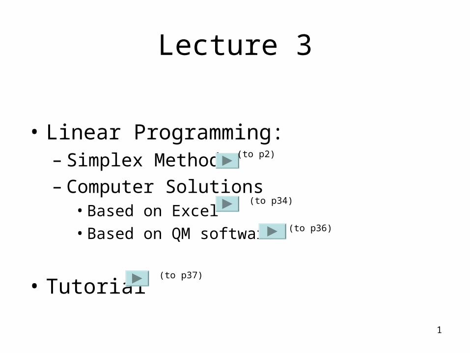
1

Lecture 3

• Linear Programming: – Simplex Method – Computer Solutions

• Based on Excel• Based on QM software

• Tutorial

(to p2)

(to p34)

(to p36)

(to p37)

2

Simplex Method

• Last week, we covered on using the graphical approach in deriving solutions for LP problem

• Question:– Can we solve all LP problems using graphical

approach ? (to p3)

3

Answer is “NO”

• Why?

Consider the following equation:

x1+x2+x3+x4 = 4

• It is extremely difficult for us to use graph to represent this equation

• Thus, we need another systematic approach to solve an LP problem – known as Simplex Method (to p4)

4

Simplex Method

• It is a method which applies Linear Algebra technique to determine values of determine values of decision variablesdecision variables of a set of equations

• Steps for simplex method

• Special/irregular cases

• Other cases

(to p1)

(to p5)

(to p24)

(to p28)

5

Steps for simplex method

• Step 1– Convert all LP resource constraints into a

standard format

• Step 2– Form a simplex tableau– Transfer all values of step 1 into the simple

tableau– Determine the optimal solution for the above

tableau by following the simplex method simplex method algorithmalgorithm

(to p4 )

(to p6)

(to p13)

(to p15)

(to p17)

6

Step 1

• Convert LP problem into standard format!

• We refer standard format here as.– All constraints are in a form of “equation” – i.e. not equation of ≥ or ≤– Procedural steps (to p7)

7

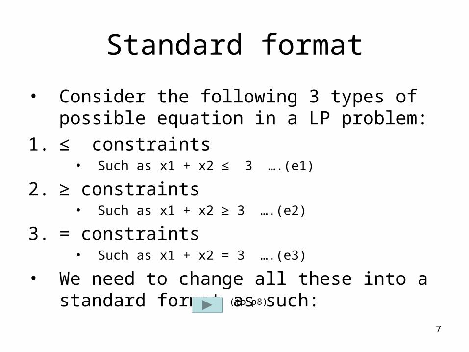
Standard format

• Consider the following 3 types of possible equation in a LP problem:

1. ≤ constraints• Such as x1 + x2 ≤ 3 ….(e1)

2. ≥ constraints• Such as x1 + x2 ≥ 3 ….(e2)

3. = constraints• Such as x1 + x2 = 3 ….(e3)

• We need to change all these into a standard format as such: (to p8)

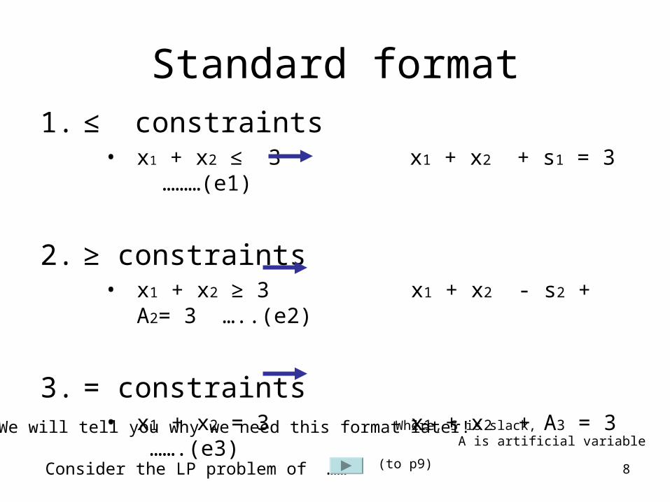
8

Standard format1. ≤ constraints

• x1 + x2 ≤ 3 x1 + x2 + s1 = 3 ………(e1)

2. ≥ constraints• x1 + x2 ≥ 3 x1 + x2 - s2 + A2= 3 …..(e2)

3. = constraints• x1 + x2 = 3 x1 + x2 + A3 = 3 …….(e3)

We will tell you why we need this format later!

Consider the LP problem of ……

Where, S is slack, A is artificial variable

(to p9)

9

Sample of an LP problem

• maximize Z=$40x1 + 50x2 subject to 1x1 + 2x2 40 ………(e1) 4x2 + 3x2 120 ……..(e2) x1 0 ……...(e3)

x2 0 ………(e4)Convert them into a standard format will be like …

(We can leave e3 and e4 alone as it is an necessary constraints for LP solution!)

More example….

(to p10)

(to p12)

10

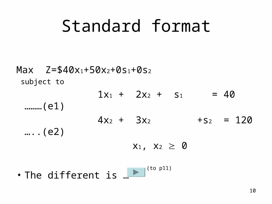
Standard format

Max Z=$40x1+50x2+0s1+0s2

subject to

1x1 + 2x2 + s1 = 40 ………(e1)

4x2 + 3x2 +s2 = 120 …..(e2)

x1, x2 0

• The different is …(to p11)

11

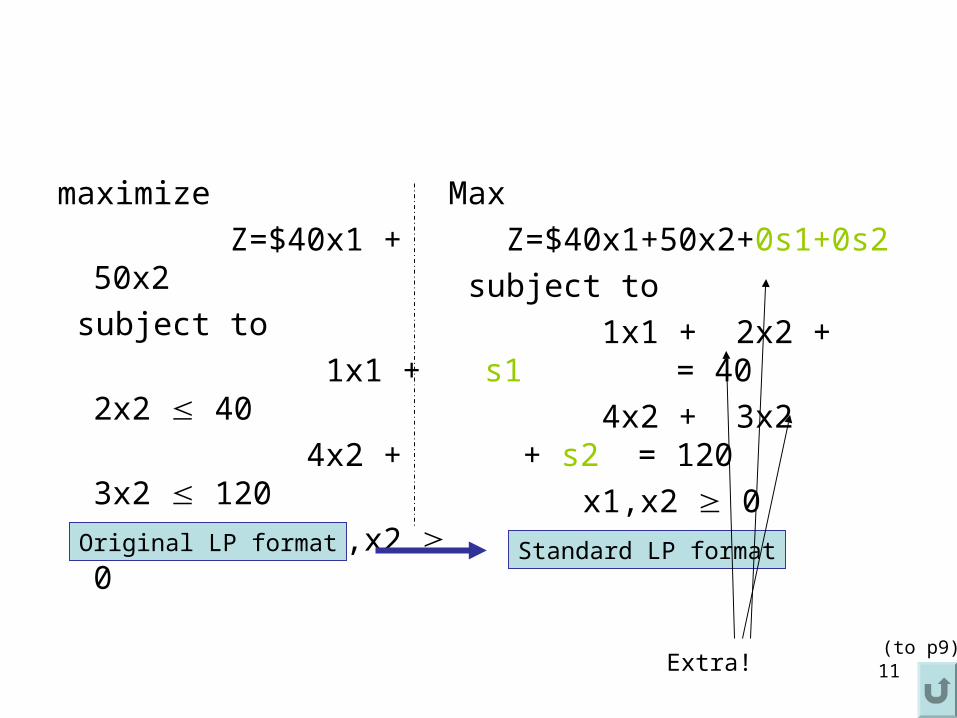
maximize

Z=$40x1 + 50x2

subject to

1x1 + 2x2 40

4x2 + 3x2 120

x1,x2 0

Max

Z=$40x1+50x2+0s1+0s2

subject to

1x1 + 2x2 + s1 = 40

4x2 + 3x2 + s2 = 120

x1,x2 0

Original LP format Standard LP format

Extra!(to p9)

12

More example of standard format

• Consider the following:

M refer to very big value, -ve value here meansthat we don’t wish to retain it in the final solution

(to p5)

13

Forming a simplex tableau

• A simple tableau is outline as follows:

What are these? (to p14)

14

Forming a simplex tableau

• A simple tableau is outline as follows:

we will discuss onhow to use them very soon!

Cost in the obj. func.

LP Decision variables

We will compute this value later It is known as marginal value

(to p5)

15

Transfer all values

Max Z=$40x1+50x2+0s1+0s2

subject to

1x1 + 2x2 + s1 = 40

4x2 + 3x2 + s2 = 120

x1,x2 0

These values read from s1 and s2 here

Basic variables(to p5)

(to p16)

16

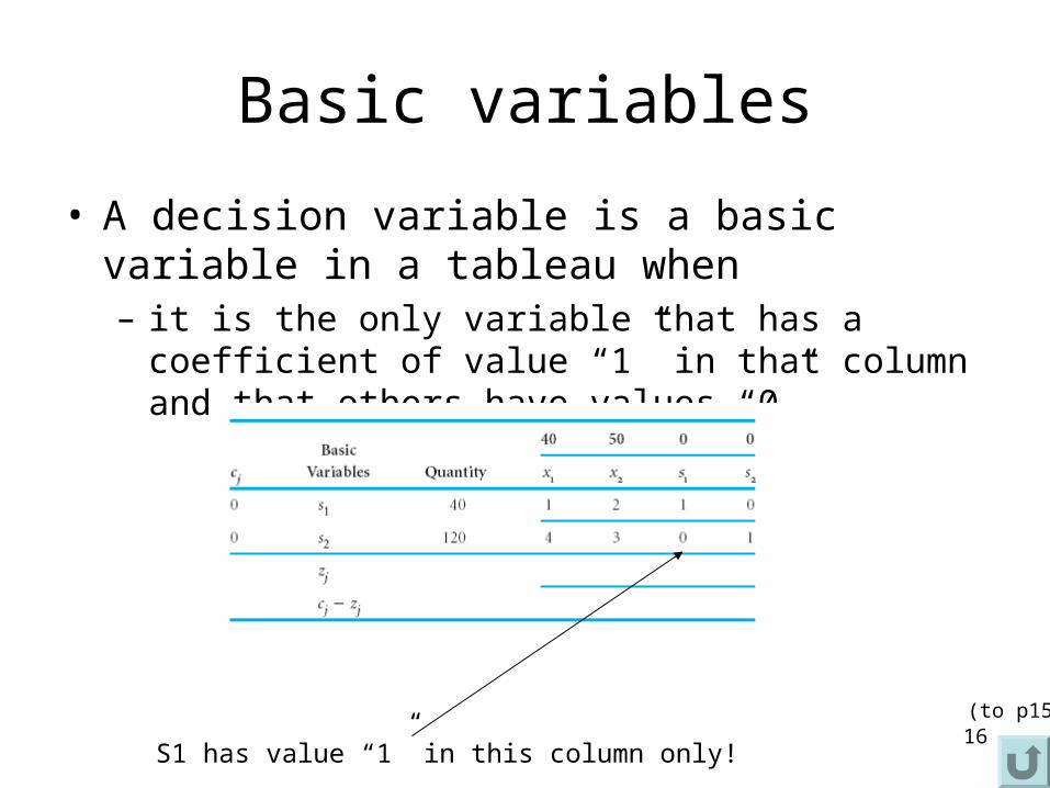
Basic variables

• A decision variable is a basic variable in a tableau when– it is the only variable that has a coefficient of value “1”

in that column and that others have values “0”

S1 has value “1” in this column only!

(to p15)

17

simplex method algorithmsimplex method algorithm

• Compute zj values• Compute cj-zj values• Determine the enteringentering variable• Determine the leavingleaving variable• Revise a new tableau

– Introducing cell that crossed by “pivot row” and “pivot column” that has only value “1” and the rest of values on that column has value “0”

• Repeat above steps until all cj-zi are all negative values– example

(to p18)

(to p19)

(to p20)

(to p22)

(to p21)

(to p23)(to p5)

18

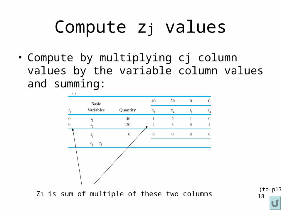
Compute zj values

• Compute by multiplying cj column values by the variable column values and summing:

Z1 is sum of multiple of these two columns(to p17)

19

Compute cj-zj values

All Cj are listed on this row

(to p17)

20

Determine the enteringentering variable• It is referred to

– The variable (i.e. the column) with the largest largest positive cpositive cjj-z-zjj value value

– Also known as “Pivot column”

Max value, ie higher marginal cost contribute to the obj fuc

This mean, we will next introduce x2 as a basic variableIn next Tableau

(to p17)

21

Determine the leavingleaving variable

• Min value of ratio of quantity values by the pivot column of entering variable

• Also known as “Pivot row”

Min value = min (40/2, 120/3) = mins (20,40), thus pick the first value

This mean, s1 will leave as basic variable in next Tableau

(to p17)

22

Revise a new tableauNote, this value is copied

This row values divided by 2

New row x 3 – old row (2), note quantity must > 0

Resume z and c-j computation!(to p17)

23

until all cj-zi are all negative values

• The following is the optimal tableau, and the solution is:

All negative values, STOP

And s1 =0 and s2= 0

(to p17)

24

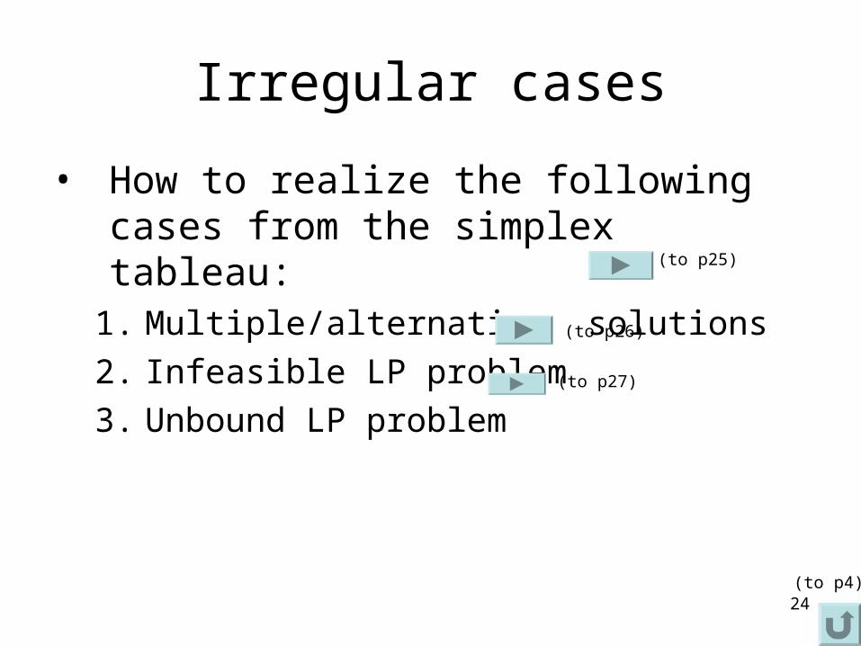
Irregular cases

• How to realize the following cases from the simplex tableau:

1. Multiple/alternative solutions

2. Infeasible LP problem

3. Unbound LP problem

(to p4)

(to p25)

(to p26)

(to p27)

25

Multiple/alternative solutions

• Alternative solution is to consider the non-basic variable that has cj-zj = 0 as the next pivot column and repeat the simplex steps

Note: S1 is not a basic variable but has value “0” for cj-zj

(to p24)

26

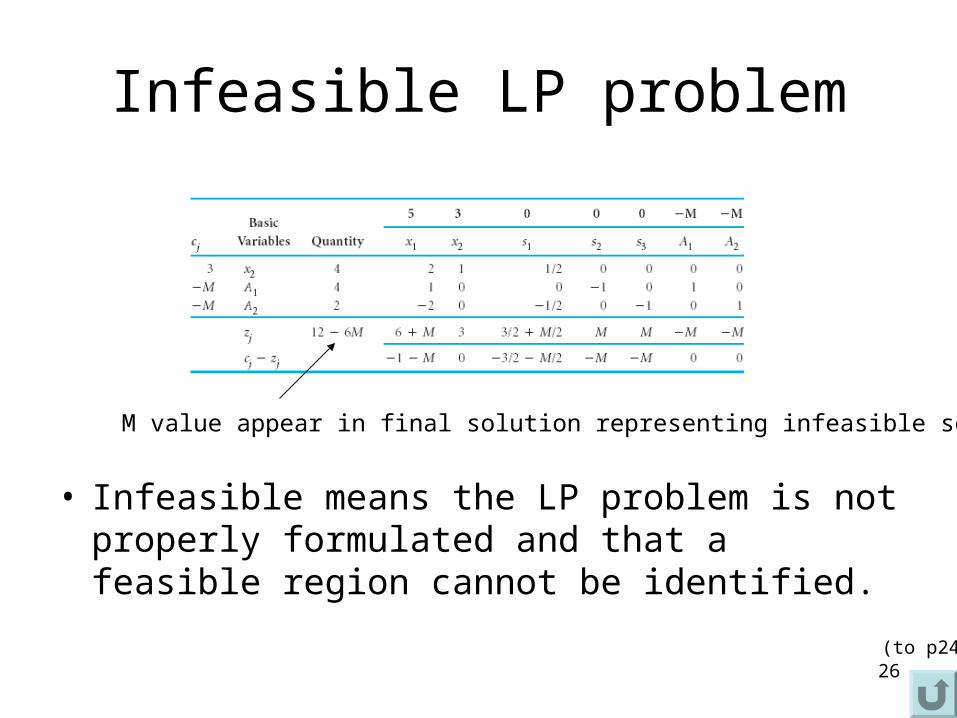
Infeasible LP problem

• Infeasible means the LP problem is not properly formulated and that a feasible region cannot be identified.

M value appear in final solution representing infeasible solution

(to p24)

27

Unbound LP problem

• Cannot identifying the Pivot row (i.e. leaving basic variable)

(for s1 as pivot column)

(to p24)

28

Other cases

1. Minimizing Z

2. When a decision variable is– either ≤ or ≥

3. Degeneracy

(to p29)

(to p32)

(to p30)

(to p4)

29

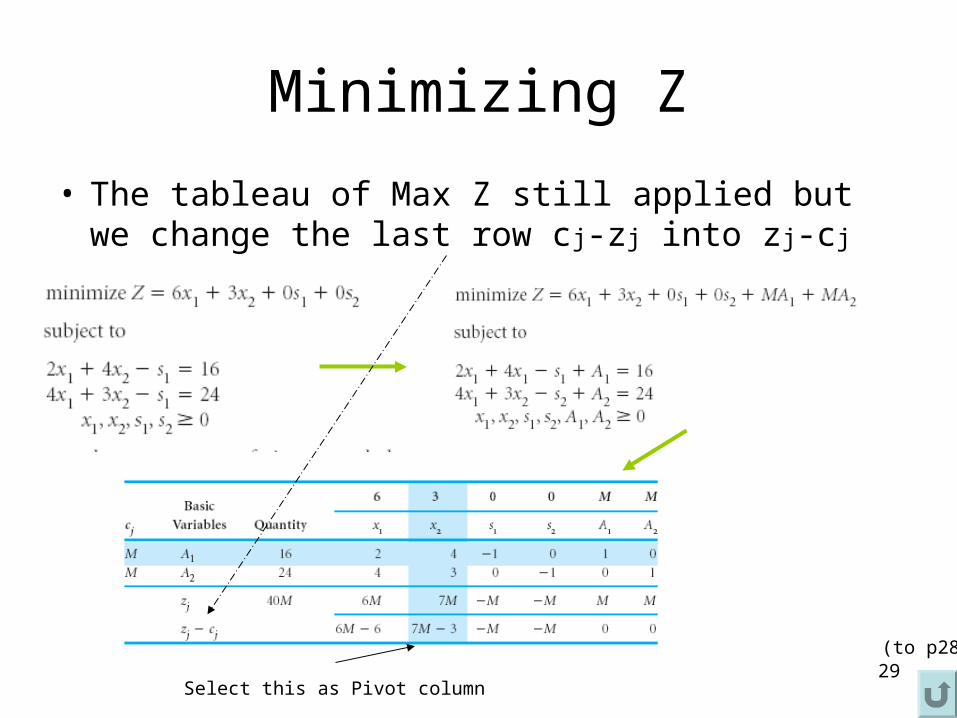
Minimizing Z

• The tableau of Max Z still applied but we change the last row cj-zj into zj-cj

Select this as Pivot column

(to p28)

30

either ≤ or ≥

If x1 is either ≤ or ≥, then

We adopt a transformation as such:let x1 = x’1 – x’’1

And then substitute it into the LP problem, and then follow the normal procedure

Example …

(to p28)

(to p31)

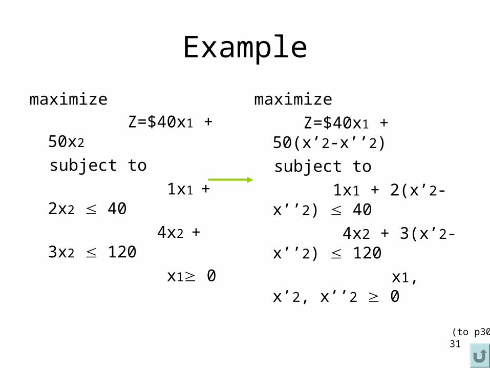
31

Example

maximize Z=$40x1 + 50x2

subject to

1x1 + 2x2 40

4x2 + 3x2 120

x1 0

maximize

Z=$40x1 + 50(x’2-x’’2)

subject to

1x1 + 2(x’2-x’’2) 40

4x2 + 3(x’2-x’’2) 120

x1, x’2, x’’2 0

(to p30)

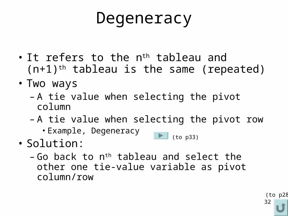
32

Degeneracy

• It refers to the nth tableau and (n+1)th tableau is the same (repeated)

• Two ways– A tie value when selecting the pivot column– A tie value when selecting the pivot row

• Example, Degeneracy

• Solution:– Go back to nth tableau and select the other

one tie-value variable as pivot column/row

(to p28)

(to p33)

33

Example, Degeneracy

Degeneracy

(to p32)

34

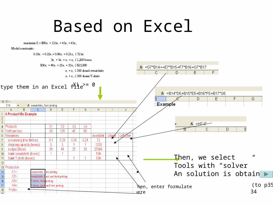
Based on Excel

Xi >= 0We type them in an Excel file

Then, enter formulatehere

Then, we select Tools with “solver”An solution is obtained

(to p35)

35

Solution using Excel

How to read them?

(to p1)

36

QM software

• Install the QM software• Loan QM software• Select option of “Linear Programming” from

the “Module”• Then select “open” from option “file” to type in a

new LP problem• Following instructions of the software

accordingly• See software illustration!

(to p1)

37

Tutorial

• Chapter 4,

• Edition 8th: #12, #17, #19

• Edition 9th: #7, #11, #12

And from appendix A/B

• P3, p20, p25, p32