Lecture 20

Continuous Problems

Linear Operators and Their Adjoints

SyllabusLecture 01 Describing Inverse ProblemsLecture 02 Probability and Measurement Error, Part 1Lecture 03 Probability and Measurement Error, Part 2 Lecture 04 The L2 Norm and Simple Least SquaresLecture 05 A Priori Information and Weighted Least SquaredLecture 06 Resolution and Generalized InversesLecture 07 Backus-Gilbert Inverse and the Trade Off of Resolution and VarianceLecture 08 The Principle of Maximum LikelihoodLecture 09 Inexact TheoriesLecture 10 Nonuniqueness and Localized AveragesLecture 11 Vector Spaces and Singular Value DecompositionLecture 12 Equality and Inequality ConstraintsLecture 13 L1 , L∞ Norm Problems and Linear ProgrammingLecture 14 Nonlinear Problems: Grid and Monte Carlo Searches Lecture 15 Nonlinear Problems: Newton’s Method Lecture 16 Nonlinear Problems: Simulated Annealing and Bootstrap Confidence Intervals Lecture 17 Factor AnalysisLecture 18 Varimax Factors, Empircal Orthogonal FunctionsLecture 19 Backus-Gilbert Theory for Continuous Problems; Radon’s ProblemLecture 20 Linear Operators and Their AdjointsLecture 21 Fréchet DerivativesLecture 22 Exemplary Inverse Problems, incl. Filter DesignLecture 23 Exemplary Inverse Problems, incl. Earthquake LocationLecture 24 Exemplary Inverse Problems, incl. Vibrational Problems

Purpose of the Lecture

Teach you a tiny bit of analysis

enough for you to understand

Linear Operators and their Adjoints

because they are the core techniqueused in the so-called

adjoint method of computing data kernels

everything we do today

is based on the idea of

generalizingdiscrete problems to continuous problems

a function

m(x)

is the continuous analog of a vector

m

a function

m(x)

is the continuous analog of a vector

m

simplification: one spatial dimension x

comparison

m is of length Mm(x) is infinite dimensional

What is the continuous analogof a matrix L ?

We’ll give it a symbol, ℒand a name, a linear operator

Matrix times a vector is another vector

b = L aso we’ll want

linear operator on a functionis another function

b(x) = ℒ a(x)

Matrix arithmetic is not communative

L(1) L(2) a ≠ L(2) L(1) a so we’ll not expect that property

for linear operators, either

ℒ (1) ℒ(2) a(x) ≠ ℒ (2) ℒ(1) a(x)

Matrix arithmetic is associative

(L(1) L(2)) L(3) a = L(1) (L(2) L(3) ) a so well want

that property for linear operators, too

(ℒ (1) ℒ(2) )ℒ(3) a(x) = ℒ (1) (ℒ(2) ℒ(3)) a(x)

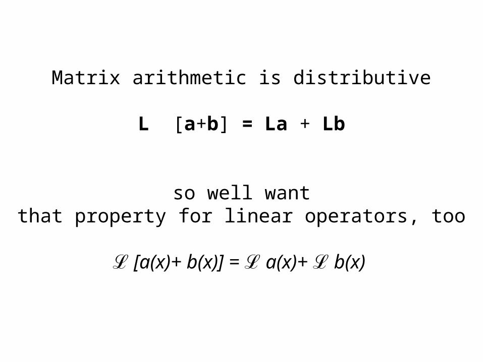
Matrix arithmetic is distributive

L [a+b] = La + Lbso well want

that property for linear operators, too

ℒ [a(x)+ b(x)] = ℒ a(x)+ ℒ b(x)

Hint to the identity of ℒmatrices can approximate

derivativesand integrals

B

LAa ≈ da/dx Laa ≈B

Linear Operatorℒany combination of functions,

derivativesand integrals

ℒ a(x)= c(x) a(x) ℒ a(x)= da/dx

ℒa(x) = b(x)da/dx + c(x) d2a/dx 2 ℒ a(x)= ∫0x a(ξ)dξ

ℒ a(x)= f(x)∫0∞ a(ξ)g(x,ξ ) dξ

all perfectly good ℒ a(x)’s

What is the continuous analogof the inverse L-1 of a matrix L ?

call it ℒ -1

ProblemLA not square, so has no inverse

derivative determines a function only up to an additive constant

Patch by adding top row that sets the constant

Now LB LC = I

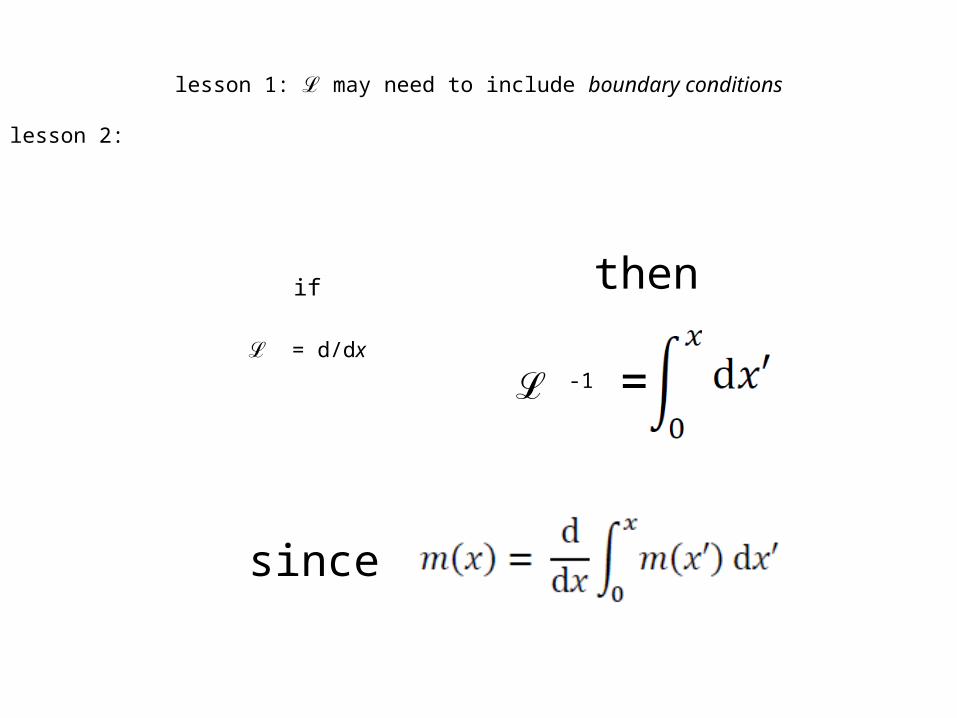
lesson 1: ℒ may need to include boundary conditions

lesson 2:

if

ℒ = d/dx ℒ -1 =

then

since

the analogy to the matrix equation

L m = fand its solution m = L-1 f

is the differential equationℒ m = fand its Green function solution

ℒ

so the inverse to a differential operator ℒ

is the Green function integral

ℒ -1 a(x) =

where F solves

a(ξ)

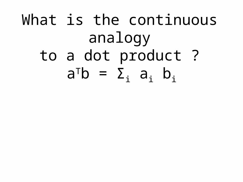
What is the continuous analogyto a dot product ?

aTb = Σi ai bi

The continuous analogyto a dot product

s = aTb = Σi ai biis the inner product

squared length of a vector

|a|2 = aTasquared length of a function

|a|2 = (a,a)

important property of a dot product

(La)T b = aT (LTb)

important property of a dot product

(La)T b = aT (LTb) what is the continuous analogy ?

(ℒa, b )= (a, ?b )

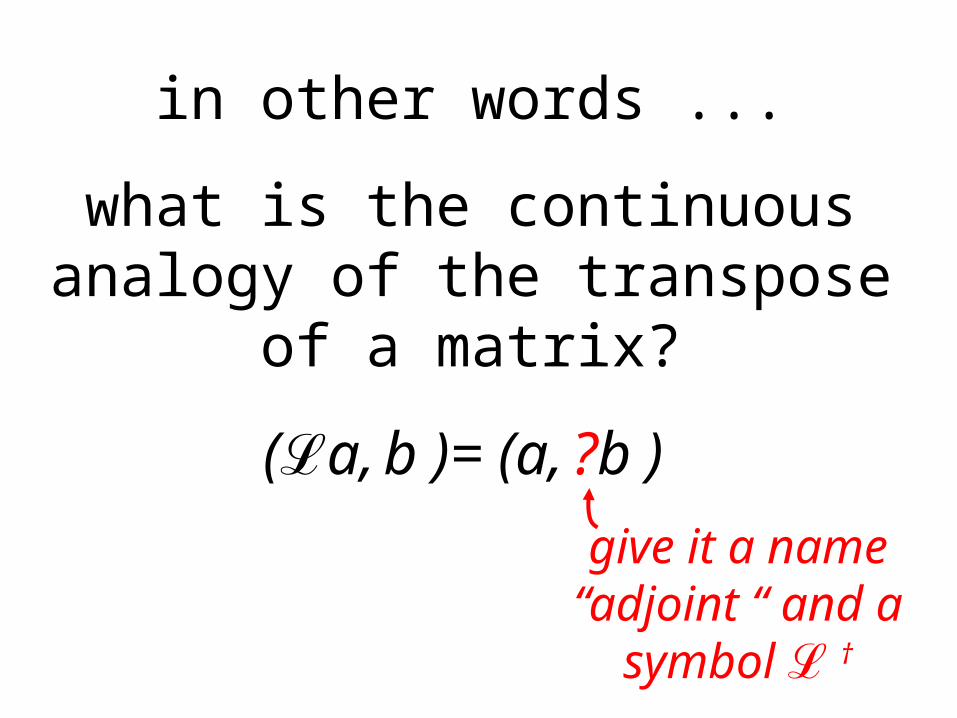
in other words ...

what is the continuous analogy of the transpose of a matrix?

(ℒa, b )= (a, ?b ) by analogy , it must be another linear operatorsince transpose of a matrix is another matrix

in other words ...

what is the continuous analogy of the transpose of a matrix?

(ℒa, b )= (a, ?b ) give it a name “adjoint “ and a symbol ℒ †

so ...

(ℒa, b )= (a, ℒ † b )

so, given ℒ, how do you determine ℒ † ?

so, given ℒ, how do you determine ℒ † ?

various ways ,,,

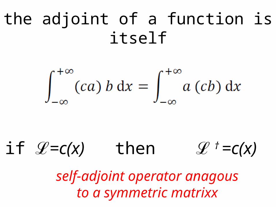
the adjoint of a function is itself

if ℒ=c(x) then ℒ † =c(x)

the adjoint of a function is itself

if ℒ=c(x) then ℒ † =c(x) a function is self-adjoint

the adjoint of a function is itself

if ℒ=c(x) then ℒ † =c(x) self-adjoint operator anagous to a symmetric matrixx

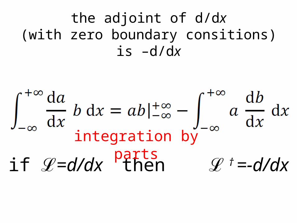
the adjoint of d/dx(with zero boundary consitions)

is –d/dx

if ℒ=d/dx then ℒ † =-d/dx

the adjoint of d/dx(with zero boundary consitions)

is –d/dx

if ℒ=d/dx then ℒ † =-d/dxintegration by parts

the adjoint of d2/dx 2 is itself

a function is self-adjoint

apply integration by parts twice

if ℒ=d2/dx 2 then ℒ † =d2/dx 2

trick using Heaviside

step function

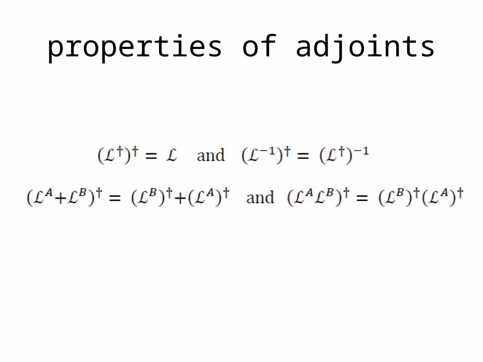
properties of adjoints

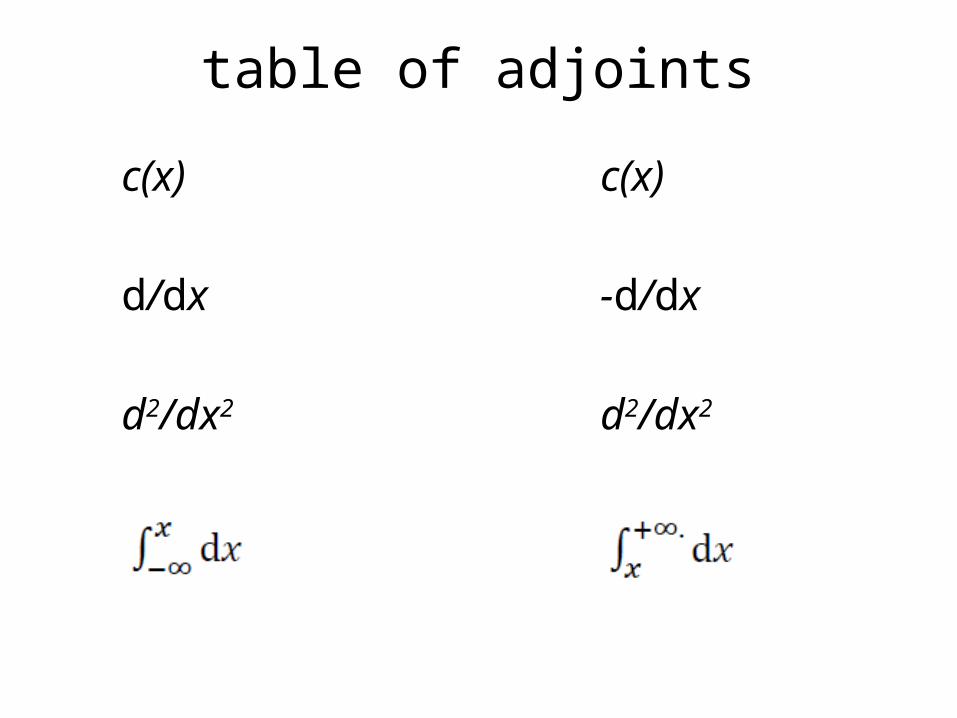
table of adjoints

c(x)-d/dxd2/dx2

c(x)d/dxd2/dx2

analogiesmLLm=fL-1f=L-1ms=aTb(La) Tb= a T(LTb)LT

m(x)ℒℒm(x)=f(x)ℒ-1f(x) =ℒ-1f(x)s=(a(x), b(x))(ℒa, b) =(a, ℒ†b)ℒ†

how is all this going to help us?

step 1

recognize thatstandard equation of inverse theory

is an inner productdi = (Gi, m)

step 2suppose that we can show thatdi = (hi, ℒm)

then do thisdi = (ℒ†hi, m)soGi = ℒ†hi

step 2suppose that we can show thatdi = (hi, ℒm)

then do thisdi = (ℒ†hi, m)soGi = ℒ†hi

formula for the data kernel