Lecture 2 Uncertainty 2

Uncertainty ContinuedLecture 2 – Tom Holden

Intermediate Microeconomics Semester 2

http://micro2.tholden.org/

ECO2051 – Intermediate Microeconomics

http://micro2.tholden.org/

Example of optimisation(For the board)

• Odds on Arsenal winning the premier league 10 to 1. You think their probability is 𝑝1.

• You have £1000 to spend on consumption if you don’t bet.

• Your von-Neumann-Morgenstern utility function is 𝑝1 𝑐1 +1 − 𝑝1 𝑐2

• How much should you bet?

• Suppose you bet 𝑥.• Consumption if Arsenal win: 𝑐1 = 1000 + 10𝑥.

• Consumption if Arsenal lose: 𝑐2 = 1000 − 𝑥.


How do we derive the budget constraint in 𝑐1, 𝑐2 space?

• 𝑐1 = 1000 + 10𝑥

• 𝑐2 = 1000 − 𝑥• So 𝑥 = 1000 − 𝑐2.

• Thus:• 𝑐1 = 1000 + 10 1000 − 𝑐2 = 11000 − 10𝑐2

• So:

• 𝑐2 =1

1011000 − 𝑐1 = 1100 −

𝑐1

10.


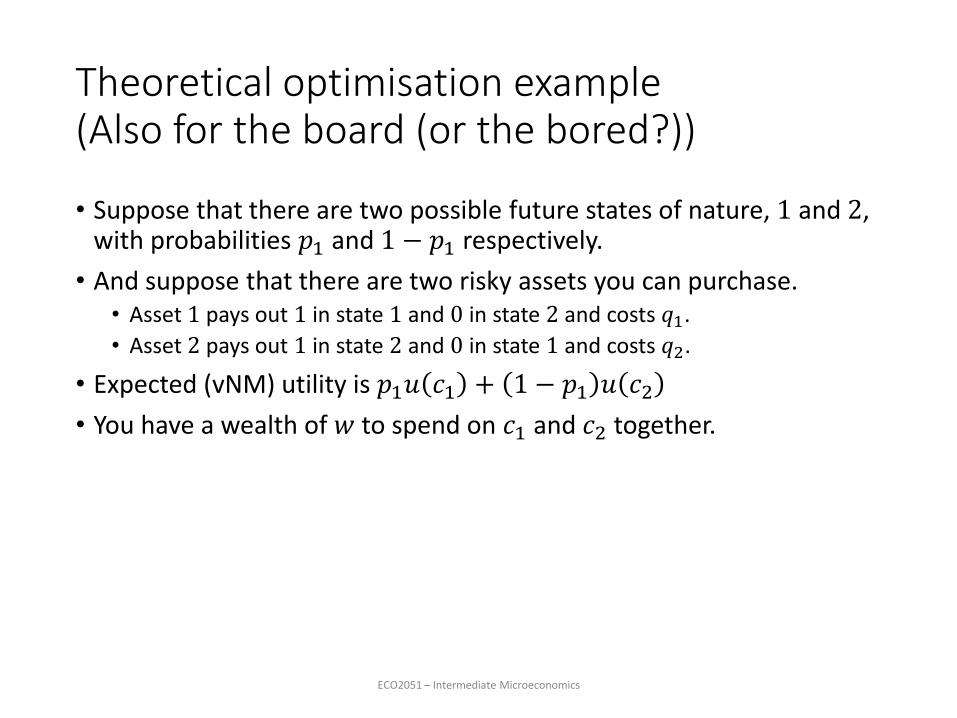
Theoretical optimisation example(Also for the board (or the bored?))

• Suppose that there are two possible future states of nature, 1 and 2, with probabilities 𝑝1 and 1 − 𝑝1 respectively.

• And suppose that there are two risky assets you can purchase.• Asset 1 pays out 1 in state 1 and 0 in state 2 and costs 𝑞1.

• Asset 2 pays out 1 in state 2 and 0 in state 1 and costs 𝑞2.

• Expected (vNM) utility is 𝑝1𝑢 𝑐1 + 1 − 𝑝1 𝑢 𝑐2

• You have a wealth of 𝑤 to spend on 𝑐1 and 𝑐2 together.


This time

• More concrete applications of expected utility theory• Insurance

• Diversification in investment

• Decisions over criminal actions


Reading

• For uncertainty:• Varian, Chapter 12 and its appendix.

• Varian, Chapter 13.

• Wikipedia: Exponential utility, Log-normal distribution

• For the welfare topic which we begin today:• Varian, Chapter 33,

• Morgan, Katz and Rosen, Chapter 12


https://en.wikipedia.org/wiki/Exponential_utility

https://en.wikipedia.org/wiki/Log-normal_distribution

Application 1: Insurance (1/6)

• Lesson: A risk averse individual offered actuarially fair insurance will always choose to fully insure.

• We have already shown that a risk averse individual won’t take a fair bet.

• Another way of saying this is that a risk averse person will avoid uncertainty if given an actuarially fair way to do so.


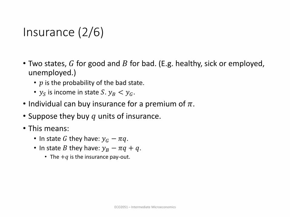
Insurance (2/6)

• Two states, 𝐺 for good and 𝐵 for bad. (E.g. healthy, sick or employed, unemployed.)• 𝑝 is the probability of the bad state.

• 𝑦𝑆 is income in state 𝑆. 𝑦𝐵 < 𝑦𝐺.

• Individual can buy insurance for a premium of 𝜋.

• Suppose they buy 𝑞 units of insurance.

• This means:• In state 𝐺 they have: 𝑦𝐺 − 𝜋𝑞.

• In state 𝐵 they have: 𝑦𝐵 − 𝜋𝑞 + 𝑞.• The +𝑞 is the insurance pay-out.


Insurance (3/6)

• Expected utility is:

• 𝑝𝑢 𝑦𝐵 − 𝜋𝑞 + 𝑞 + 1 − 𝑝 𝑢 𝑦𝐺 − 𝜋𝑞

• FOC 𝑞: 0 = 𝑝 1 − 𝜋 𝑢′ 𝑦𝐵 − 𝜋𝑞 + 𝑞 − 1 − 𝑝 𝜋𝑢′ 𝑦𝐺 − 𝜋𝑞

• So: 𝑢′ 𝑦𝐵−𝜋𝑞+𝑞

𝑢′ 𝑦𝐺−𝜋𝑞=𝜋 1−𝑝

𝑝 1−𝜋


Insurance (4/6)

• Suppose there are many such consumers, and they all face idiosyncratic risks.• I.e. risks are uncorrelated across individuals.

• Also assume each individual has the same exogenous risk.

• I.e. we rule out any problems with:• Moral hazard (insured people take less care).• Adverse selection (only risky people insure).

• Then although each individual is risky, if an insurance company is insuring many individuals their returns will not be risky.• A proportion 𝑝 of them will encounter the bad state and make a claim.


Insurance (5/6)

• Expected profit for the insurance company is:

• 𝑝 𝜋𝑞 − 𝑞 + 1 − 𝑝 𝜋𝑞 = 𝜋 − 𝑝 𝑞

• With a competitive market, entry occurs until profits equal zero.• Hence 𝜋 = 𝑝.

• So in this case the consumer FOC becomes:

• 𝑢′ 𝑦𝐵 − 𝜋𝑞 + 𝑞 = 𝑢′ 𝑦𝐺 − 𝜋𝑞


Insurance (6/6)

Endowment

Good SoW

𝑦𝐵

𝑦𝐺

The budget constraint has slope −𝜋

1−𝜋

The indifference curve has slope −𝑝𝑢′ 𝑦𝐵−𝜋𝑞+𝑞

1−𝑝 𝑢′ 𝑦𝐺−𝜋𝑞

Bad SoW

What happens if insurance companies make a profit?

Good SoW

𝑦𝐺 B

B’

IC

IC’

Bad state of the world 𝑦𝐵

A risk averse individualwill still insure, but notfully.

In budget line B the consumer faces a premium

𝜋 = 𝑝 = 0.4 so slope is −0.4

0.6= −

2

3

In budget line B’ the consumer faces a premium 𝜋 = 0.5 so the slope is −1.

Endowment

Application 2: Investment

• Lessons:• Riskier assets must have higher expected returns.

• Investors can be thought of as balancing risk and return.

• Investors will generally seek to diversify.

• The stock market and mutual funds are examples of how the market provides diversification through the stock market.


Diversion: log-normal distributions

• Suppose that a random variable 𝑋 is normally distributed with mean 𝜇 and standard deviation 𝜎.• I.e. 𝑋~N 𝜇, 𝜎2

• Then if we define a new random variable by 𝑌 = exp𝑋, then 𝑌 has the “log-normal” distribution.

• Useful fact: 𝔼𝑌 = exp 𝜇 +1

2𝜎2

• exp𝑋 is not a linear function, so 𝔼 exp𝑋 ≠ exp 𝔼𝑋


Exponential utility (1/4)

• Suppose:• My utility is: 𝑢 𝑥 = 1 − exp −𝑎𝑥 .

• Asset 𝑅 (for risky) gives a normally distributed return with mean 𝜇𝑅 and standard deviation 𝜎𝑅, and costs 𝑝𝑅. Call the (unknown, random) realisation of this return 𝑥𝑅.

• Asset 𝑆 (for safe) gives a guaranteed return of 𝜇𝑆 and costs 𝑝𝑆.

• My income (to spend on the two assets) is 𝑌.

• I buy 𝑞𝑅 units of the risky asset and 𝑞𝑆 units of the safe asset.



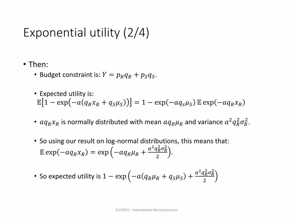
• Then:• Budget constraint is: 𝑌 = 𝑝𝑅𝑞𝑅 + 𝑝𝑆𝑞𝑆.

• Expected utility is:𝔼 1 − exp −𝑎 𝑞𝑅𝑥𝑅 + 𝑞𝑆𝜇𝑆 = 1 − exp −𝑎𝑞𝑠𝜇𝑆 𝔼 exp −𝑎𝑞𝑅𝑥𝑅

• 𝑎𝑞𝑅𝑥𝑅 is normally distributed with mean 𝑎𝑞𝑅𝜇𝑅 and variance 𝑎2𝑞𝑅2𝜎𝑅

2.

• So using our result on log-normal distributions, this means that:

𝔼exp −𝑎𝑞𝑅𝑥𝑅 = exp −𝑎𝑞𝑅𝜇𝑅 +𝑎2𝑞𝑅

2𝜎𝑅2

2.

• So expected utility is 1 − exp −𝑎 𝑞𝑅𝜇𝑅 + 𝑞𝑆𝜇𝑆 +𝑎2𝑞𝑅

2𝜎𝑅2

2



• Lagrangian:

• ℒ = 1 − exp −𝑎 𝑞𝑅𝜇𝑅 + 𝑞𝑆𝜇𝑆 +𝑎2𝑞𝑅

2𝜎𝑅2

2− 𝜆 𝑝𝑅𝑞𝑅 + 𝑝𝑆𝑞𝑆 − 𝑌

• Define: 𝑘 = −𝑎 𝑞𝑅𝜇𝑅 + 𝑞𝑆𝜇𝑆 +𝑎2𝑞𝑅

2𝜎𝑅2

2, so:

• ℒ = 1 − exp 𝑘 − 𝜆 𝑝𝑅𝑞𝑅 + 𝑝𝑆𝑞𝑆 − 𝑌

• FOC 𝑞𝑅: 0 = 𝑎𝜇𝑅 − 𝑎2𝑞𝑅𝜎𝑅

2 exp𝑘 − 𝜆𝑝𝑅.

• FOC 𝑞𝑆: 0 = 𝑎𝜇𝑆 exp 𝑘 − 𝜆𝑝𝑆.



• Equating 𝜆 in the two FOCs gives: 𝑝𝑅

𝑝𝑆=𝜇𝑅−𝑎𝑞𝑅𝜎𝑅

2

𝜇𝑆.

• Thus, 𝑞𝑅 =𝜇𝑆

𝑎𝜎𝑅2

𝜇𝑅

𝜇𝑆−𝑝𝑅

𝑝𝑆.

• As the relative return of the risky asset increases, or its relative price falls, more of it is purchased.

• As the risky asset gets riskier, or risk aversion increases, less of the risky asset is purchased.

• Also, from the budget constraint: 𝑝𝑅𝜇𝑆

𝑎𝜎𝑅2

𝜇𝑅

𝜇𝑆−𝑝𝑅

𝑝𝑆+ 𝑝𝑆𝑞𝑆 = 𝑌.

• Hence, 𝑞𝑆 =𝑌

𝑝𝑆−𝑝𝑅

𝑝𝑆

𝜇𝑆

𝑎𝜎𝑅2

𝜇𝑅

𝜇𝑆−𝑝𝑅

𝑝𝑆.


Diversification (1/2)

• An investor is choosing between two risky assets. • Sun screen – pays 7% if sunny, nothing if rainy.

• Umbrellas – pays 7% if rainy, nothing if sunny.

• Sun and rain have a 50: 50 chance.

• If I put £100 in either, I get an expected return of £3.50.

• If I put £50 in each, get £3.50 for certain.

• A risk averse person will get a higher utility if they diversify.


Diversification (2/2)

• In the previous example it is very clear that the return on the two assets is perfectly negatively correlated. • This is why it works.

• When seeking to diversify investors want assets which do not follow the same trends.• ‘Beta’ measures how closely correlated an assets return is with the rest of

the stock market.

• Measured by regression of asset value on value of stock market as a whole.

• Assets with low betas are sought after.

• Mutual funds or trackers are a way for the general investor to keep a diversified portfolio.


The stock market

• The stock market allows the original owners of a firm to convert the risky position of having all their wealth tied into one asset into cash which they can invest more widely.

• Shareholders can buy and sell shares depending on the policies of the companies and the amount of risk they are prepared to bear.

• Ownership of risky assets is moved from those who are risk averse to those who are somewhat less risk averse.

• It allows investors to diversify.


Decisions over criminal actions (1/2)

• Suppose I’m considering becoming a burglar, to supplement my meagre university salary.

• There is an infinite variety of houses I could break into, indexed by the amount I could sell the jewellery they contain for.

• If I successfully steal 𝑣 thousand pounds of jewellery, my utility is 𝑢 𝑣 = 1 + 𝑣.

• But the more jewellery a house contains, the more likely I am to get caught.

• Assume that the probability of getting caught while breaking into a house containing 𝑣thousand pounds worth of jewellery is 𝑝 𝑣 = 1 −

1

1+𝑣.

• If I get caught, I’ll be locked up, giving me a utility of 𝑢𝑐 ≥ 0.

• If I don’t burgle a house assume I get utility of 1.000…01 with certainty.• So I prefer not to burgle any house to burgling a house with no jewellery.


Decisions over criminal actions (2/2)

• Should I burgle a house? If so, which?

• Assume I steal from a house containing 𝑣 thousand pounds of jewellery.• My expected utility is:

1 − 𝑝 𝑣 𝑢 𝑣 + 𝑝 𝑣 𝑢𝑐 =1 + 𝑣

1 + 𝑣+ 1 −

1

1 + 𝑣𝑢𝑐

• Slightly tricky to maximise. FOC implies 𝑣∗ = −1 + 4𝑢𝑐2.

• But I’ll only burgle a house if 𝑣∗ > 0. I.e. if 𝑢𝑐2 >

1

4i.e. if 𝑢𝑐 >

1

2(as we

are assuming 𝑢𝑐 > 0).• So if punishment is strong I won’t burgle.


Summary of Uncertainty

• A risk averse person will always seek to insure if an actuarially fair policy is offered.

• A risk averse person will seek to diversify whenever possible.

• Risky investments will generally pay more.


Welfare preview (1/2)

• Imagine you did not know who you were going to be born as. (But you were conscious in this strange ethereal state.) And you were asked to allocate (say) income across individuals.

• Given your ignorance, you might assume that it was equally likely you could be born as anyone.

• Thus your expected utility is just 1

𝑛 𝑈𝑖 where 𝑛 is the number of

individuals, and 𝑈𝑖 is the utility you would have if you were born as individual 𝑖.

• Imagine for simplicity that your utility as agent 𝑖 is just some function 𝑢 𝑌𝑖 of your income 𝑌𝑖 as 𝑖.


Welfare preview (2/2)

• Suppose incomes distributions have to be within some set of possibilities.• E.g. 𝑌1 = 10, 𝑌2 = 1 , 𝑌1 = 2, 𝑌2 = 2

• If the function 𝑢 was linear (so risk neutral) which income distribution would you prefer?

• If the function 𝑢 was highly risk averse which would you prefer?

• Inequality aversion and risk aversion are closely tied.


Lecture 2 Uncertainty 2

Documents

Transcript of Lecture 2 Uncertainty 2