System Identification

Lecture 2:Models of linear time-ectu e 2: ode s o ea t einvariant systems

Sahar Moghimi

1

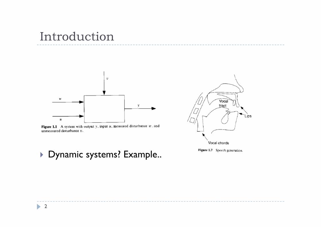
IntroductionIntroduction

Dynamic systems? Example..

2

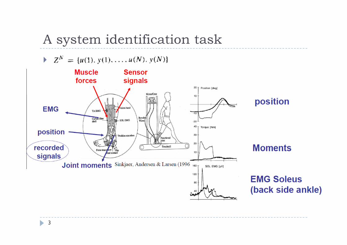
A system identification taskA system identification task

3

A system identification taskA system identification task

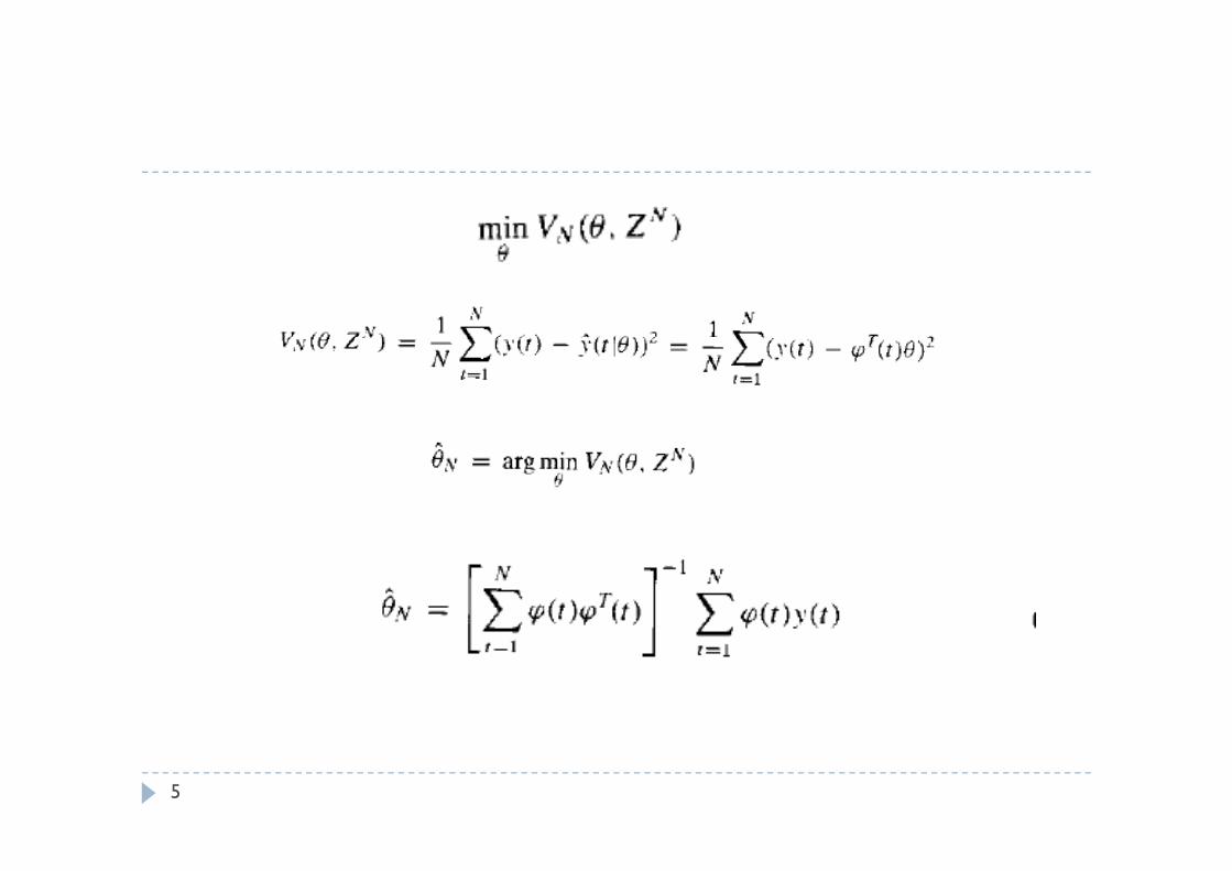
Linear regressionLinear regression

Regressor vector

4

5

System identification steps:System identification steps: A data set A set of candidate models (model structure) A rule for determination of model parametersp

6

Review chapters

2: Time-invariant linear systemsy 3: Simulation and prediction

7

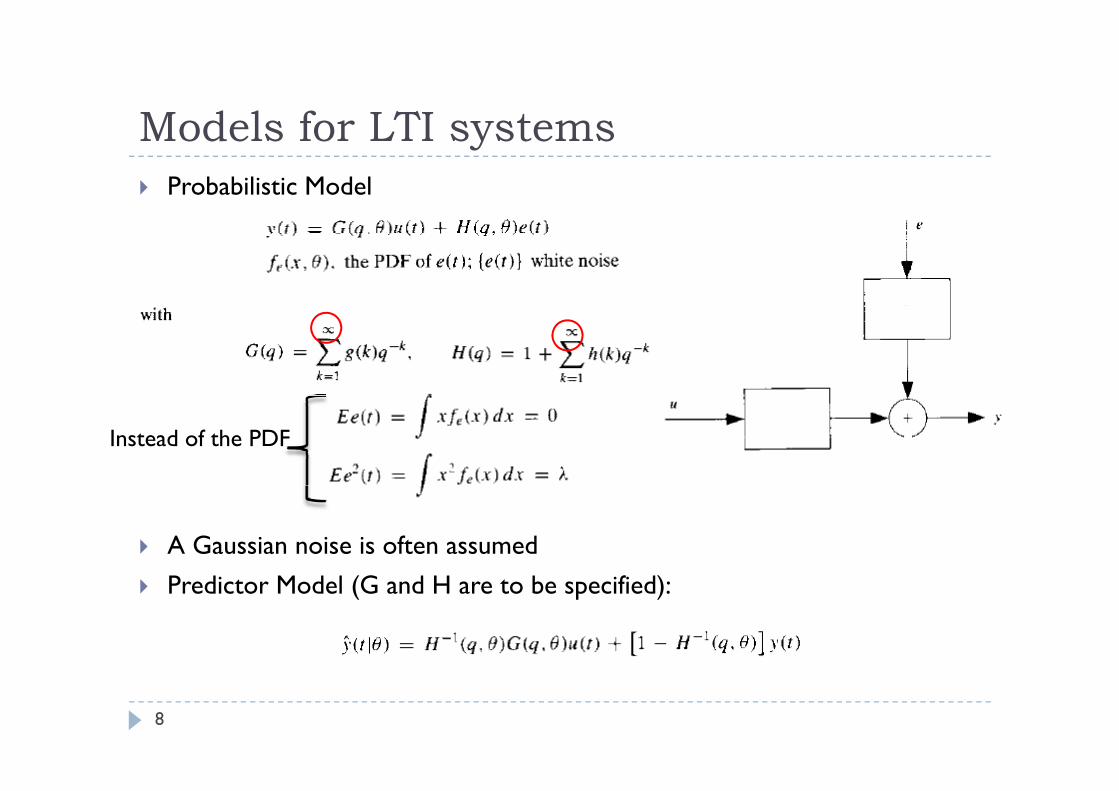
Models for LTI systemsModels for LTI systems Probabilistic Model

Instead of the PDF

A Gaussian noise is often assumed Predictor Model (G and H are to be specified):

8

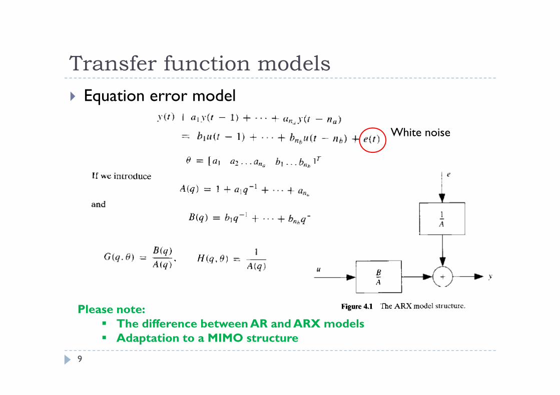
Transfer function modelsTransfer function models Equation error model

White noise

Please note: The difference between AR and ARX models

9

Adaptation to a MIMO structure

Example: NIRS study of musical emotions

10

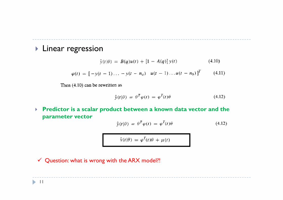
Linear regression

Predictor is a scalar product between a known data vector and the parameter vector

Question: what is wrong with the ARX model?!

11

The disadvantage of the ARX model

Disturbances are part of the system dynamics.

The transfer function of the deterministic part G of the system and the transfer function of the stochastic part H of the system have the same set of poles. This coupling can be unrealistic.

The system dynamics and stochastic dynamics of the system do not share the same set of poles all the time.

H d hi di d if h d i l However, you can reduce this disadvantage if you have a good signal-to-noise ratio.

12

ARMAX:

13

Pseudo-linear regression

Please note that B determined the dynamic of the system, sometimes there is a delay between u and y so B starts from a value other than 1: Exampleis a delay between u and y so B starts from a value other than 1: Example

Unavailable values can be set to zero

14

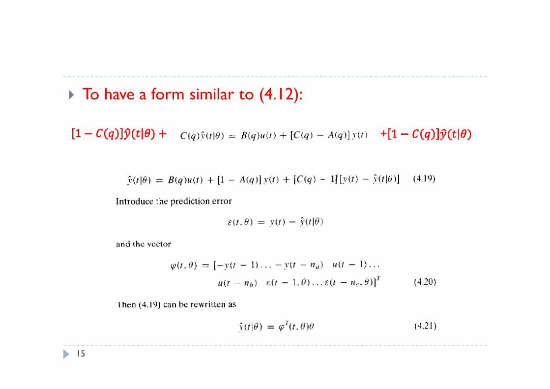
To have a form similar to (4.12):

15

Least square from text Will be introduced with details in the third lecture

16

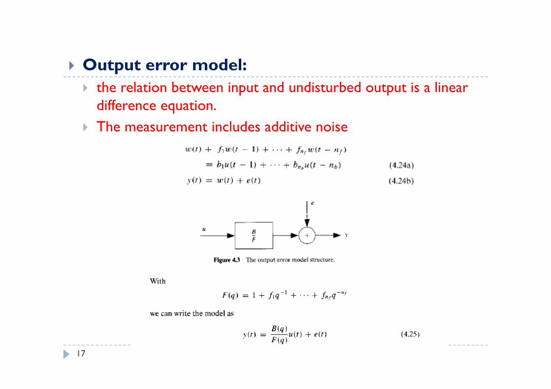
O t t d l Output error model: the relation between input and undisturbed output is a linear

difference equation difference equation. The measurement includes additive noise

17

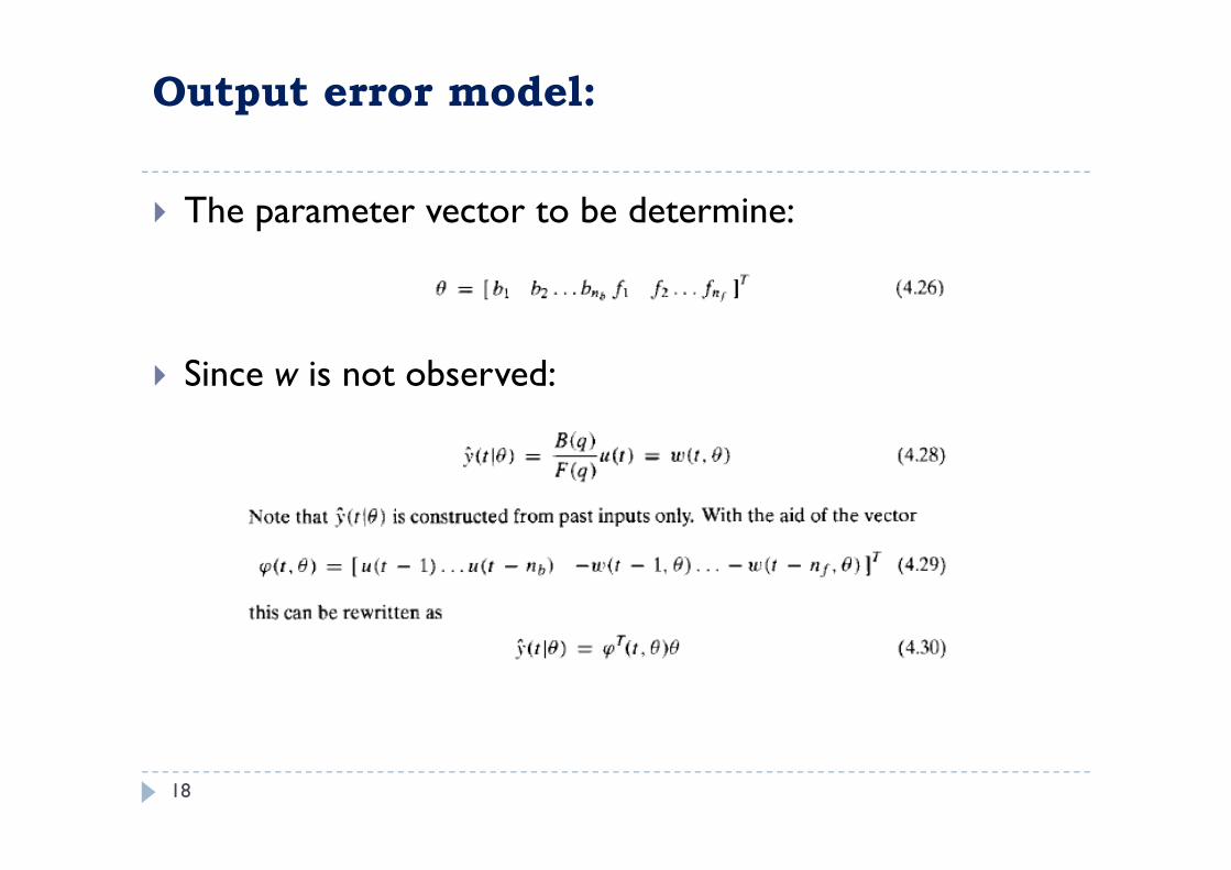
Output error model:

The parameter vector to be determine:

Since w is not observed:

18

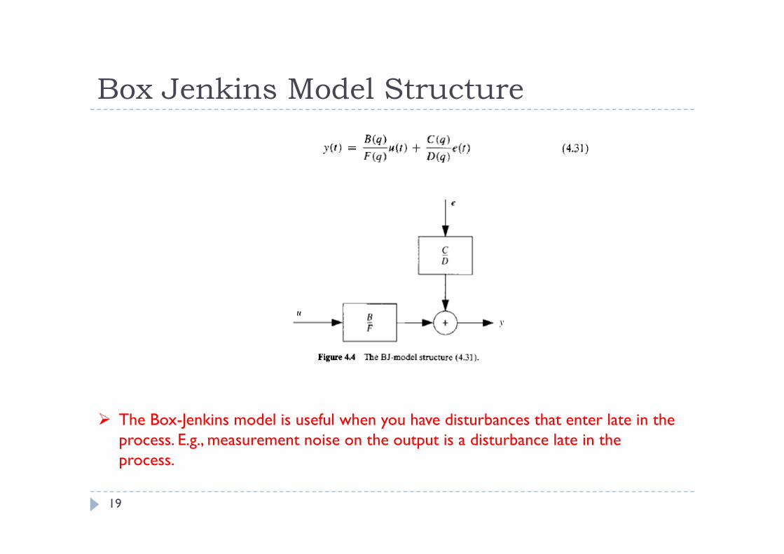
Box Jenkins Model StructureBox Jenkins Model Structure

The Box-Jenkins model is useful when you have disturbances that enter late in the process. E.g., measurement noise on the output is a disturbance late in the process.

19

p

General structure:

20

PLEASE NOTE!PLEASE NOTE! For any particular problem the choice of the

model structure to use depends on the dynamics and the noise characteristics of the system.

Using a model with more freedom or parameters is not always better as it can result in the

d li f i d i d i modeling of nonexistent dynamics and noise characteristics. Thi i h h i l i i h i i This is where physical insight into a system is helpful.

21

Choose a data set Divide it to estimation and test sets Define the mentioned models and use LSE to evaluate

your model. Analyze your estimation errory y

22

State space modelsState space models States variables are usually chosen with an insight to the

physical properties of the system

Measurement

23

State space modelsState space models The following equations describe a state-space model in

discrete time.

x(t) is the state vector, y(t) is the system output, u(t) the system input and v(t) is the stochastic error. A, B, and C are the system matrices.

24

Assumed:Measured:

Further modeling of the noise term

25

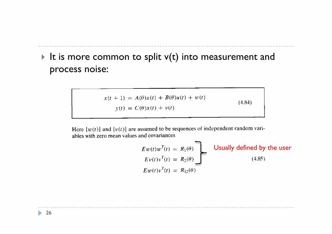
It is more common to split v(t) into measurement and process noise:

Usually defined by the user

26

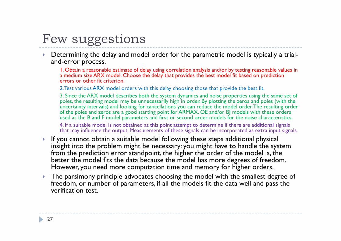
Few suggestionsFew suggestions Determining the delay and model order for the parametric model is typically a trial-

and-error process. 1. Obtain a reasonable estimate of delay using correlation analysis and/or by testing reasonable values in a medium size ARX model. Choose the delay that provides the best model fit based on prediction errors or other fit criterion.2. Test various ARX model orders with this delay choosing those that provide the best fit.3. Since the ARX model describes both the system dynamics and noise properties using the same set of poles, the resulting model may be unnecessarily high in order. By plotting the zeros and poles (with the uncertainty intervals) and looking for cancellations you can reduce the model order. The resulting order of the poles and zeros are a good starting point for ARMAX, OE and/or BJ models with these orders used as the B and F model parameters and first or second order models for the noise characteristics.4. If a suitable model is not obtained at this point attempt to determine if there are additional signals that may influence the output. Measurements of these signals can be incorporated as extra input signals.

If you cannot obtain a suitable model following these steps additional physical insight into the problem might be necessary: you might have to handle the system insight into the problem might be necessary: you might have to handle the system from the prediction error standpoint, the higher the order of the model is, the better the model fits the data because the model has more degrees of freedom. However, you need more computation time and memory for higher orders.

Th i i i l d t h i th d l ith th ll t d f The parsimony principle advocates choosing the model with the smallest degree of freedom, or number of parameters, if all the models fit the data well and pass the verification test.

27

ReferenceReference Chapter 1-4, System Identification: Theory for Users,

Ljung

28

Any questions?Any questions?

29