Lecture #2 Maxwell’s Equations - Home - Home | EM Labemlab.utep.edu/ee5390cem/Lecture 2 --...
32
9/15/2017 1 Lecture 2 Slide 1 EE 5337 Computational Electromagnetics Lecture #2 Maxwell’s Equations These notes may contain copyrighted material obtained under fair use rules. Distribution of these materials is strictly prohibited Instructor Dr. Raymond Rumpf (915) 747‐6958 [email protected] Outline • Maxwell’s equations • Physical Boundary conditions • Parameter relations • Preparing Maxwell’s equations for CEM • The wave equation and its solutions • Scaling properties of Maxwell’s equations Lecture 2 Slide 2
Transcript of Lecture #2 Maxwell’s Equations - Home - Home | EM Labemlab.utep.edu/ee5390cem/Lecture 2 --...

9/15/2017
1
Lecture 2 Slide 1
EE 5337
Computational Electromagnetics
Lecture #2
Maxwell’s Equations
These notes may contain copyrighted material obtained under fair use rules. Distribution of these materials is strictly prohibited
InstructorDr. Raymond Rumpf(915) 747‐[email protected]
Outline
• Maxwell’s equations
• Physical Boundary conditions
• Parameter relations
• Preparing Maxwell’s equations for CEM
• The wave equation and its solutions
• Scaling properties of Maxwell’s equations
Lecture 2 Slide 2

9/15/2017
2
Lecture 2 Slide 3
Maxwell’s Equations
Born
Died
June 13,1831Edinburgh, Scotland
November 5, 1879Cambridge, England
James Clerk Maxwell
Lecture 2 Slide 4
Sign Conventions for Waves
To describe a wave propagating the positive z direction, we have two choices:
, cosE z t A t kz
, cosE z t A t kz
Most common in engineering
Most common science and physics
Both are correct, but we must choose a convention and be consistent with it. For time‐harmonic signals, this becomes
expE z A jkz
expE z A jkz
Negative sign convention
Positive sign convention

9/15/2017
3
Lecture 2 Slide 5
Summary of Sign Conventions
Lecture 2 Slide 6
Summary of Sign Conventions

9/15/2017
4
Lecture 2 Slide 7
Lorentz Force Law
F qE qv B
Magnetic ForceElectric Force
One additional equation is needed to completely describe classical electromagnetism...
Lecture 2 Slide 8
Alternate Forms of Maxwell’s Equations
Maxwell’s Equations with Gaussian Units
0
1free2 0
F J
e F J D
Relativistic Maxwell’s Equations
Maxwell’s Equations in Moving Media
0
0
14
14 4
1
v
v
BD E B v
c t
DB H J D v
c t
0
0
14
14 4
v
v
BD E
c t
DB H J
c t

9/15/2017
5
Lecture 2 Slide 9
Time‐Harmonic Maxwell’s Equations
Time‐Domain
0
v
BD E
t
DB H J
t
Frequency‐Domain(e+jkz convention)
0vD E j B
B H J j D
Frequency‐Domain(e-jkz convention)
0vD E j B
B H J j D
Lecture 2 Slide 10
Gauss’s Law
Electric fields diverge from positive charges and converge on negative charges.
vD
yx zDD D
Dx y z
If there are no charges, electric fields must form loops.

9/15/2017
6
Lecture 2 Slide 11
Gauss’s Law for Magnetism
Magnetic fields always form loops.
0B
yx zBB B
Bx y z
Lecture 2 Slide 12
Consequence of Zero DivergenceThe divergence theorems force the D and B fields to be perpendicular to the propagation direction of a plane wave.
k D
0
0jk r
D
de
d
no charges
0
0
jk d
k d
k
k
k B
0
0jk r
B
be
b
no charges
0
0
jk b
k b
k
k

9/15/2017
7
Lecture 2 Slide 13
Ampere’s Law with Maxwell’s Correction
DH J
t
ˆ ˆ ˆy yx xz zx y z
H HH HH HH a a a
y z z x x y
Circulating magnetic fields induce currents and/or time varying electric fields.
Currents and/or time varying electric fields induce circulating magnetic fields.
H
DJ
t
Lecture 2 Slide 14
Faraday’s Law of Induction
BE
t
ˆ ˆ ˆy yx xz zx y z
E EE EE EE a a a
y z z x x y
Circulating electric fields induce time varying magnetic fields.Time varying magnetic fields induce circulating electric fields.
E
B t

9/15/2017
8
Lecture 2 Slide 15
Consequence of Curl Equations
The curl equations predict electromagnetic waves!!
Electric Field
Magnetic Field
Lecture 2 16
The Constitutive Relations
Electric Response
ED
Magnetic Response
HB
• Electric field intensity (V/m)• Initial electric “push.”• Induced electric field.• Electric energy in vacuum.
• Permittivity (F/m)• Measure of how well a material stores electric energy.
• Electric flux density (C/m2)• Pretends as if all electric energy is displaced charge.
• Includes electric energy in vacuum and matter.
• Magnetic field intensity (A/m)• Initial magnetic “push.”• Induced magnetic field.• Magnetic energy in vacuum.
• Permeability (H/m)• Measure of how well a material stores magnetic energy.
• Magnetic flux density (Wb/m2)• Pretends as if all magnetic energy is tilted magnetic dipoles.
• Includes magnetic energy in vacuum and matter.

9/15/2017
9
Lecture 2 17
Material Classifications
Linear, isotropic and non‐dispersive materials:
Dispersive materials:
D t E t
Anisotropic materials:
D t t E t
D t E t
Nonlinear materials:
1 2 32 30 0 0e e eD t E t E t E t
We will use this almost exclusively
A key point is that you can wrap all of the complexities associated with modeling strange materials into this single equation. This will make your code more modular and easier to modify. It may not be as efficient as it could be though.
Lecture 2 18
Types of Anisotropy
D t E t
B t H t
Isotropic
D t E t
B t H t
Anisotropic
D t E t
B t H t
Gryrotropic
D t E t H
B t H t E
Bi‐Isotropic Bi‐Anisotropic
aa ab ac
ba bb bc
ca cb cc
aa ab ac
ba bb bc
ca cb cc
electrically anisotropic magnetically anisotropic
1 2
2 1
3
0
0
0 0
j
j
1 2
2 1
3
0
0
0 0
j
j
gyroelectric gyromagnetic
D t E t H
B t H t E
iso
iso iso
iso
0 0
0 0
0 0
o
o
e
0 0
0 0
0 0
0 0
0 0
0 0
a
b
c
isotropic
uniaxial
biaxial

9/15/2017
10
Lecture 2 Slide 19
All Together Now…
Divergence Equations
0
v
B
D
DH J
t
BE
t
Curl Equations
Constitutive Relations
D t t E t
B t t H t
What produces fields
How fields interact with materials
means convolution
means tensor
Lecture 4 Slide 20
Maxwell’s Equations in Cartesian Coordinates (1 of 4)Vector Terms
ˆ ˆ ˆ
ˆ ˆ ˆ
x x y y z z
x x y y z z
E E a E a E a
D D a D a D a
ˆ ˆ ˆ
ˆ ˆ ˆ
x x y y z z
x x y y z z
H H a H a H a
B B a B a B a
ˆ ˆ ˆx x y y z zJ J a J a J a
Divergence Equations
0
0yx z
D
DD D
x y z
0
0yx z
B
BB B
x y z

9/15/2017
11
Lecture 4 Slide 21
Maxwell’s Equations in Cartesian Coordinates (2 of 4)Constitutive Relations
D E
ˆ ˆˆ ˆˆˆy y yx x xx x xy y xz zz z zx x zy y zx x yyx y z zy zy zzD D a Ea E ED a E E EE aa a E E
y yx x y
z zx x
x xx x xy y xz z
zy y zz z
y y yz zD E E
D E
D E E E
E
E E
B H x xx x xy y xz z
y yx x yy y yz z
z zx x zy y zz z
B H H H
B H H H
B H H H
Lecture 4 Slide 22
Maxwell’s Equations in Cartesian Coordinates (3 of 4)Curl Equations
BE
t
ˆ ˆ ˆ ˆ ˆ ˆy yx xz zx y z x x y y z z
E EE EE Ea a a B a B a B a
y z z x x y t
ˆ ˆ ˆˆ ˆˆy xzx x
yx zy
y x zz zy
E E Ba a
E BEa
BE Ea a
y z tx tx ya
z t
y x
z
z
x
z
yx
yE BE
y z t
BE E
zE E B
x y
x t
t

9/15/2017
12
Lecture 4 Slide 23
Maxwell’s Equations in Cartesian Coordinates (4 of 4)Curl Equations
DH J
t
y
yx zy
y x zz
xzx
DH HJ
z x tH H D
Jx y
H DHJ
y z
t
t
ˆ ˆ ˆ ˆ ˆ ˆ ˆ ˆ ˆy yx xz zx y z x x y y z z x x y y z z
H HH HH Ha a a J a J a J a D a D a D a
y z z x x y t
ˆ ˆˆ ˆ ˆˆy x zy xzx xz z
zy y y z
yx
xDH H
a J az x t
H DHa J a
y z t
H H Da J a
x y t
Lecture 4 Slide 24
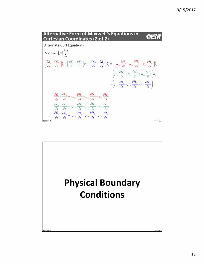
Alternative Form of Maxwell’s Equations in Cartesian Coordinates (1 of 2)Alternate Curl Equations
EHt
ˆ
ˆ
ˆ
ˆ
ˆ ˆx zy
y
y xz
yx zzx zy zz
y yxz zx xx xy x
x
z x
zyx yy yz y
z
H EEH EH Ha
z x
E
H Ha
x y
EE Ea
t t t
E Ea
a az
t t
y t
t
t t
yx xz zyx yy y
y yx x zzx zy
y yxz zxx
zz
y
z
x xz
EH EH E
z x tH EH E E
x y t
H EEH E
y z
t
t
t
t t t
t
9/15/2017
13
Lecture 4 Slide 25
Alternative Form of Maxwell’s Equations in Cartesian Coordinates (2 of 2)Alternate Curl Equations
HEt
ˆ
ˆˆ ˆ
ˆ
ˆ x y xz
y
y yxz zx xx xy xz
zy
yx zyx yy yz
x zzx zy zz
x
y
z
E EE HHE Ha aa
x y
E
y z t t t
Ea
z x
HH Ha
HH Ha
t t
t
t
t t
yx
y yx
x
y yx x z
z zxx x
zx zy zz
z zyx yy z
y z
y
x
E HE
HE HE H
z x t
H H
x y t t
E HHE
t
H
t
y t t t
t
z
Lecture 2 Slide 26
Physical Boundary Conditions

9/15/2017
14
Lecture 2 Slide 27
Physical Boundary Conditions
Tangential components of E and Hare continuous across an interface.
1,TE 2,TE
1,TH 2,TH
1 1 and 2 2 and
E and H fields normal to the interface are discontinuous across an interface.
Note: Normal components of Dand B are continuous across the interface.
1 1,NE
1 1,NH
2 2,NE
2 2,NH These are more complicated boundary conditions, physically and analytically.
1,Tk 2,TkTangential components of the wave vector are continuous across an interface.
1,ND
1,NB
2,ND
2,NB
Lecture 2 Slide 28
Parameter Relations

9/15/2017
15
Lecture 2 Slide 29
Map of Parameter Relations
E
H
n
0
r
0
r
0
D
B
f
0c
v
0 P
M
Lecture 2 Slide 30
The Relative Permittivity
0 r 12
0 8.854187817 10 F m
The dielectric constant of a material is its permittivity relative to the permittivity of free space.
1 r r is the relative permittivity or dielectric constant
The permittivity is a measure of how well a material stores electric energy. A circulating magnetic field induces an electric field at the center of the circulation in proportion to the permittivity.
EH
t
j

9/15/2017
16
Lecture 2 Slide 31
The Relative Permeability
0 r 6
0 1.256637061 10 H m
The relative permeability of a material is its permeability relative to the permeability of free space.
1 r r is the relative permeability
The permeability is a measure of how well a material stores magnetic energy. A circulating electric field induces a magnetic field at the center of the circulation in proportion to the permeability.
HE
t
j
Lecture 2 Slide 32
Conductivity
H J j D
Conductivity is the measure of a material’s ability to support electric current. This term is responsible for ohmic loss in materials.
It appears in Ampere’s Circuit Law.
The current density is related to conductivity and the electric field intensity through Ohm’s Law.
J E
J

9/15/2017
17
Lecture 2 Slide 33
’-j’’ Vs. and
H j j E
H E j E
It is redundant to have a complex dielectric constant along with a conductivity term, although it happens. We should use either a complex dielectric constant or a real dielectric constant and a conductivity.
j j j
jj
Lecture 2 Slide 34
Material ImpedanceThe material impedance is the parameter which describes the balance between the electric and magnetic field amplitudes.
0r
r
E H
It is calculated from the permeability and permittivity of the material.
0 free space impedance
376.73031346177
E
H k
j
Phase between E and H
Amplitude between E and H
Reactive component
Resistive component.Impedance tells us that E and H are three orders of magnitude different.
H
E

9/15/2017
18
Lecture 2 Slide 35
The Complex Refractive Index
r rn
The permittivity and permeability appear in Maxwell’s equations so they are the most fundamental material properties. However, it is difficult to determine physical meaning from them in terms of how waves propagate (i.e. speed, loss, etc.). In this case, the refractive index is a more meaningful quantity.
In the frequency‐domain, the refractive index is a complex quantity.
on n j no is the ordinary refractive index. It quantifies how quickly a wave propagates.
is the extinction coefficient. It quantifies loss and how quickly a wave decays. 0
0jk nzE z E e
* Note: when only the refractive index n is specified for a material, assume r = 1.0.
Lecture 2 Slide 36
The Complex Propagation Constant,
0zE z E e
The propagation constant is very close to the complex refractive index. It describes the speed and decay of a wave.
The propagation constant has a real and imaginary part.
j is the attenuation coefficient. It quantifies how quickly the amplitude of a wave decays.
is the propagation constant. It quantifies how quickly a wave accumulates phase. 0
z j zE z E e e
It is related to the complex refractive index through
0jk n

9/15/2017
19
Lecture 2 Slide 37
The Absorption Coefficient,
0zP z P e
The absorption coefficient describes how quickly the power in a wave decays.
WARNING: Notice the unfortunate reuse of the symbol for two different things. This is easily confused!!
The attenuation coefficient and absorption coefficient are related through
abs att2
The absorption coefficient and extinction coefficient are related through
abs 02k
Lecture 2 Slide 38
Loss Tangent
Sometimes material loss is given in terms of a “loss tangent.”
Recall that interpreting wave properties (velocity and loss) is not intuitive using just the complex dielectric function. To do this, we preferred the complex refractive index.
It turns out that the loss tangent and the extinction coefficient are essentially the same.
tan
abs
0
2
n k n
It is called a loss tangent because it is the angle in the complex plane formed between the resistive component and the reactive component of the electromagnetic field.
or
or
00
k nzP z P e

9/15/2017
20
Lecture 2 Slide 39
versus f
is the angular frequency measured in radians per second. It relates more directly to phase and k. Think cos(t).
f is the ordinary frequency measured in cycles per second. It relates more directly to time. Think cos(2ft) and =1/f.
2 f
Lecture 2 Slide 40
Wavelength and Frequency
The frequency f and free space wavelength 0 are related through
0 0c f
Inside a material, the wave slows down according to the refractive index as follows.
0cvn
m0 s299792458 speed of light in vacuumc

9/15/2017
21
Lecture 2 Slide 41
Summary of Parameter Relations
Permittivity
0
120 8.854187817 10 F m
r
Permeability
0
60 1.256637061 10 H m
r
Refractive Index Impedance
r rn 0
0 0 0 376.73031346177
r r
Wave Velocity
0
0 299792458 m s
cv
nc
Exact
Frequency and Wavelength
0 0
2 f
c f
00
Wave Number
2k
Lecture 2 Slide 42
Table of Dielectric Constants and Loss Tangents
Constantine A. Balanis, Advanced Engineering Electromagnetics, Wiley, 1989.

9/15/2017
22
Lecture 2 Slide 43
Table of Permeabilities
Constantine A. Balanis, Advanced Engineering Electromagnetics, Wiley, 1989.
Lecture 2 44
Duality Between E‐D and H‐B
Electric Field Magnetic Field
E H
D B
P M
ε μ

9/15/2017
23
Lecture 2 Slide 45
Preparing Maxwell’s Equations
for CEM
Lecture 2 Slide 46
Simplifying Maxwell’s Equations
0
0
B
D
H D t
E B t
D t t E t
B t t H t
1. Assume no charges or current sources: 0, 0v J
0
0
H
E
H j E
E j H
3. Substitute constitutive relations into Maxwell’s equations:
Note: It is useful to retain μ and ε and not replace them with refractive index n.
0
0
B
D
H j D
E j B
D E
B H
2. Transform Maxwell’s equations to frequency‐domain:Convolution becomes simple multiplication
Note: We have chose to proceed with the negative sign convention.

9/15/2017
24
Lecture 2 Slide 47
Isotropic Materials
xx xy xz xx xy xz
yx yy yz yx yy yz
zx zy zz zx zy zz
For anisotropic materials, the permittivity and permeability terms are tensor quantities.
For isotropic materials, the tensors reduce to a single scalar quantity.
0 0 0 0
0 0 0 0
0 0 0 0
Maxwell’s equations can then be written as
0
0
r
r
H
E
0
0
r
r
H j E
E j H
0 and 0 dropped from these equations because they are constants and do not vary spatially.
Lecture 2 Slide 48
Expand Maxwell’s Equations
Divergence Equations
0
0
r
r yr x r z
H
HH H
x y z
0
0
0
0
r
yzr x
x zr y
y xr z
E j H
EEj H
y z
E Ej H
z xE E
j Hx y
Curl Equations
0
0
r
r yr x r z
E
EE E
x y z
0
0
0
0
r
yzr x
x zr y
y xr z
H j E
HHj E
y z
H Hj E
z xH H
j Ex y

9/15/2017
25
Lecture 2 Slide 49
Normalize the Magnetic Field
0 rE j H
0 rH j E
Standard form of “Maxwell’s Curl Equations”
Normalized Magnetic Field
377E
nH
0
0
H j H
Normalized Maxwell’s Equations
0 rE k H
0 rH k E
0 0 0k Note:
Equalizes E and H amplitudes•Eliminates j•No sign inconsistency• Just have k0
Lecture 2 Slide 50
Starting Point for Most CEM
0
0
0
yzxx x
x zyy y
y xzz z
HHk E
y z
H Hk E
z x
H Hk E
x y
0
0
0
yzxx x
x zyy y
y xzz z
EEk H
y z
E Ek H
z xE E
k Hx y
0
0
negative sign convnetion
positive sign convnetion
j HH
j H
We arrive at the following set of equations that are the same regardless of the sign convention used.
The manner in which the magnetic field is normalized does depend on the sign convention chosen.

9/15/2017
26
Lecture 2 Slide 51
The Wave Equation and Its Solutions
Lecture 2 Slide 52
Derivation of the Wave Equation
We start with Maxwell’s curl equations.
0 rE j H
0 rH j E
Equation (1) is solved for the magnetic field.
Eq. (1) Eq. (2)
0 r
jH E
Eq. (3)
Equation (3) is substituted into Eq. (2).
00
20
1
rr
rr
jE j E
E k E

9/15/2017
27
Lecture 2 Slide 53
Two Different Wave Equations
We can derive a wave equation for both E and H.
1 2 1 20 0 r r r rE k E H k H
It is not actually possible to simplify these equations further without making an approximation. Assuming a linear homogeneous isotropic (LHI) material, the wave equations reduce to
20 r rH k H
H
2 20
2 20 0
r r
r r
H k H
H k H
20 r rE k E
E
2 20
2 20 0
r r
r r
E k E
E k E
We see that these equations will have the same solution since it is the same differential equation! So, we only have to solve one of them.
Lecture 2 Slide 54
Plane Wave Solution in Homogeneous Media
Given the wave equation in an LHI material,
2 20 0r rE k E
The solution is a plane wave.
0
0
exp
exp
E r E jk r
H r H jk r

9/15/2017
28
Lecture 2 Slide 55
Amplitude Relation
Given plane wave functions of the form
0
0
exp
exp
E r E jk r
H r H jk r
The amplitudes are related through Maxwell’s equations.
0
0 0 0
0 0 0
0 0 0
r
jk r jk rr
jk r jk rr
r
E j H
E e j H e
j k E e j H e
k E H
0 00
0 0 0r r
k E k EH
k
Lecture 2 Slide 56
IMPORTANT: Plane Waves are of Infinite Extent
Many times we just draw rays or sometime rays with perpendicular lines to represent the wave fronts.
ray ray + perpendicular lines
Unfortunately, this suggests the wave is confined spatially. In reality, plane waves are of infinite extent. Think more this way…

9/15/2017
29
Lecture 2 Slide 57
Solving the Wave Equation as a Scattering Problem
Scattering problems cast the wave equation into the following matrix form.
• A source b is needed • Only one solution exists
1 20r rE k E g
Ax b
1 20
r rk
E g
A
x b
Lecture 2 Slide 58
Solving the Wave Equation as an Eigen‐Value Problem
• No source is needed • Multiple solutions exist
The wave equation can also be solved as an eigen‐value problem. This approach is used when “modes” are being calculated.
1 20r rE k E
Ax Bx1
20
r r
E k
A B
x

9/15/2017
30
Lecture 2 Slide 59
Wave Equation Vs. Maxwell’s Equations
Wave Equation Maxwell’s Equations
1 20
1 20
r r
r r
E k E
H k H
The most generalized wave equations are
In LHI materials, these reduce to
2 20
2 20
0
0
r r
r r
E k E
H k H
Today, it is rare to see the wave equations solved in this form because it leads to spurious solutions.
The “fixes” to the spurious solutions problem are incorporated into Maxwell’s equations before a wave equation is derived.
00
0 0
0 0
yzyzxx xxx x
x xz zyy y yy y
y x y xzz z zz z
HHEE k Ek Hy zy z
E HE Hk H k E
z x z xE E H Hk H k Ex y x y
Maxwell’s equations expanded into Cartesian coordinates are
These are often written in matrix form as
0 0
0 00 0 0 0
0 0 0 0 0 0
0 0 0 0 0 0
z y z yx xx x x xx x
y yy y y yyz x z x
z zz z z zzy x y x
E H H E
E k H H k
E H H
y
z
E
E
Typically, “fixes” are incorporated here and then a wave equation is derived.
1
20
0 00 0 0 0
0 0 0 0 0 0
0 0 0 0 0 0
z y z yxx x xx x
yy y yy yz x z x
zz z zz zy x y x
E E
E k E
E E
Lecture 2 Slide 60
Scaling Properties inMaxwell’s Equations

9/15/2017
31
Lecture 2 Slide 61
Scaling Properties of Maxwell’s Equations
There is no fundamental length scale in Maxwell’s equations.
Devices may be scaled to operate at different frequencies just by scaling the mechanical dimensions or material properties in proportion to the change in frequency.
This assumes it is physically possible to scale systems in this manner. In practice, building larger or smaller features may not be practical. Further, the properties of the materials may be different at the new operating frequency.
Lecture 2 Slide 62
Scaling Dimensions
We start with the wave equation and write the parameters dependence on position explicitly.
20 0
1r
r
E r r E rr
Next, we scale the dimensions by a factor a.
20 0
1r
r
a a E r a r a E r ar a
The scale factors multiplying the operators are moved to multiply the frequency term.
2
0 0
1r
r
E r r E rr a
1 stretch dimensions
1 compress dimensions
a
a
The effect of scaling the dimensions is just a shift in frequency.
rr
a

9/15/2017
32
Lecture 2 Slide 63
Visualization of Size Scaling
fc = 500 MHz
a = 1.0
fc = 1000 MHz
a = 0.5
Lecture 2 Slide 64
Scaling and We apply separate scaling factors to and .
20 0
1r
r
E a Ea
The scale factors are moved to multiply the frequency term.
2
0 0
1r
r
E a a E
The effect of scaling the material properties is just a shift in frequency.