Lecture 2. Data Compression for One Variable

George Duncan90-786 Intermediate Empirical Methods for Public Policy and

Management

Lecture 2: Data Compression for One Variable

Forms of data compression Complex thinking about simple means Links between centers and spreads Use of Minitab

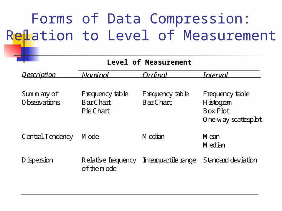
Forms of Data Compression: Relation to Level of Measurement

Description Nominal Ordinal Interval Summary of Observations

Frequency table Bar Chart Pie Chart

Frequency table Bar Chart

Frequency table Histogram Box Plot One-way scatterplot

Central Tendency Mode Median Mean Median

Dispersion Relative frequency of the mode

Interquartile range Standard deviation

Level of Measurement

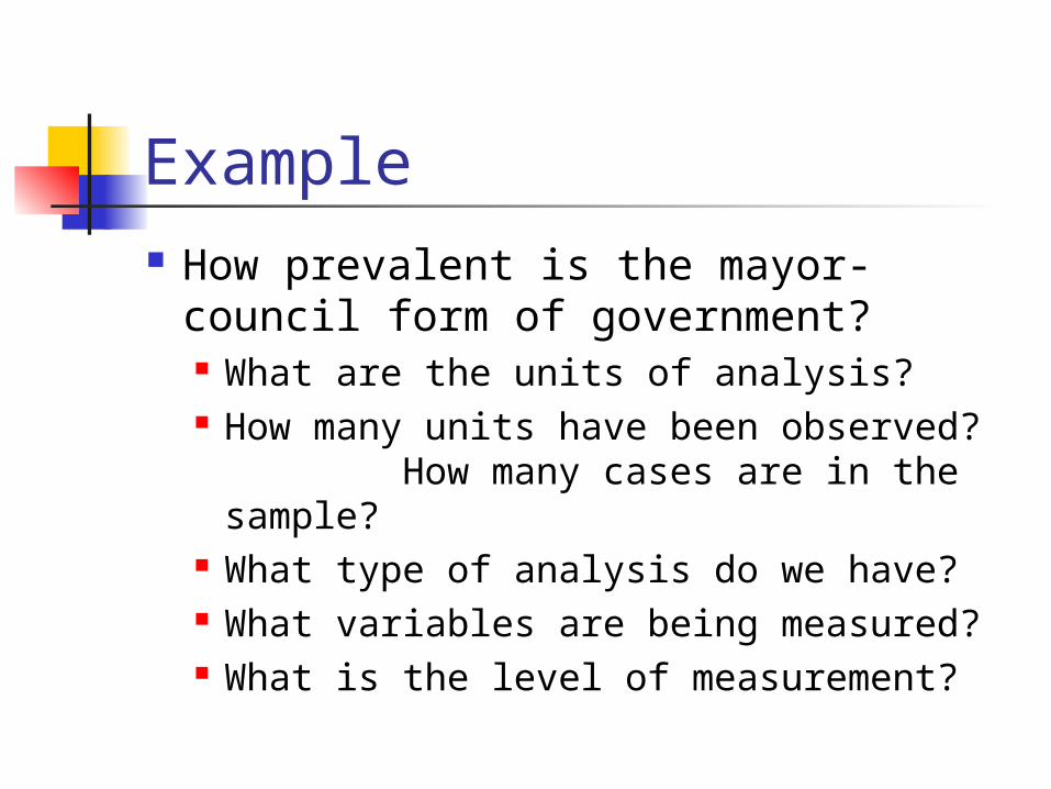
Example How prevalent is the mayor-council

form of government? What are the units of analysis? How many units have been observed?

How many cases are in the sample? What type of analysis do we have? What variables are being measured? What is the level of measurement?

Form of Government in Cities Under 25,000 Population in Kansas

No. City Symbolic Code Numerical Code

1 Abilene CM 12 Andale MC 23 Andover MC 24 Atchison CM 15 Beloit MC 26 Cherryvale CO 3

74 Winfield CM 1

Form of Government

... ... ... ...

CM = 1, council-managerMC = 2, mayor-councilCO = 3, commission

Governance Frequency Table

Value Form of Government AbsoluteFrequency

Relative Frequency

Number ofObservations

Proportion Percentage

1 Council-Manager 37 0.50 50%

2 Mayor-Council 32 0.43 43.2%

3 Commission 5 0.07 6.8%

Total 74 1.00 100%

Governance Bar Chart

0

5

10

15

20

25

30

35

40

Council-Manager Mayor-Council Commission

Governance Pie Chart

1. Council-manager 50% (37)

2. Mayor-council 43.2% (32)

3. Commission 6.8% (5)

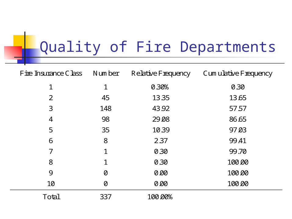
Quality of Fire Departments

Fire Insurance Class Number Relative Frequency Cumulative Frequency

1 1 0.30% 0.30

2 45 13.35 13.65

3 148 43.92 57.57

4 98 29.08 86.65

5 35 10.39 97.03

6 8 2.37 99.41

7 1 0.30 99.70

8 1 0.30 100.00

9 0 0.00 100.00

10 0 0.00 100.00

Total 337 100.00%

Fire Insurance Bar Chart

0

20

40

60

80

100

120

140

160

1 2 3 4 5 6 7 8 9 10

Garbage Collection

Tons of Garbage Number ofObservations

50-60 1560-70 2570-80 30

80-90 20

90-100 10

Total 100

Tons of Trash Collected by the City of Normal, Oklahoma for the Week of June 8, 1992

Garbage Histogram

50-60 60-70 70-80 80-90 90-100

30

25

20

15

10

5

0

Frequency

Tons of Garbage

Measures of Central Tendency

Median = 73 tons Mode = 75 tons Mean (average of all observed

values ) x = 72.97

x = x i

nWhere:

Measures of Dispersion

S =2 (x - x)

2

i

n - 1

Variance = S

Standard Deviation = S

Range = Max - Min2

where:

Coefficient of Variation = Sx

Measure of Dispersion: Garbage Example

Range = 97 - 50 = 47

Variance = 151.3

Standard Deviation = 12.3

Coefficient of Variation = 0.17

Box Plot

Median

Q 25th percentile

Q 75th percentile

1

3

Whisker

Whisker

Interquartile range, IQR = ( Q - Q )

13

o Outlier (extreme data value)

Inner fence = Q - 1.5 *IQR1

Inner fence = Q + 1.5 *IQR3

Outer fence = Q - 3.0 *IQR1

Outer fence = Q + 3.0 *IQR3

Garbage Box Plot

Median = 73

Q = 64

Q = 82.25

Max = 97

Min = 50

1

3

Shapes of Distribution

Positive skewness Mean > Median

Symmetric distribution Mean = Median

Negative skewness Mean < Median

Complex Thinking about Simple Means

The mean time served for drug law violation by prisoners released from U.S. Federal prisons during 1965 to 1980 was 22.4 months.

The median family income in Texas in

1975 was $12,672. The modal number of commercial TV

stations in 1980 among the fifty U.S. states was 12 per state.

Applications of a Mean Earnings of workers in the automobile industry averaged $577.30 per week in the U.S. for

1986. The mean temperature in Minneapolis-St. Paul during January is minus 12 degrees Celsius. The U.S. national rate of motor-vehicle traffic deaths per 100,000 population in 1985 was

18.8.

As a simple example, if a y-batch is the numbers 2, 6, and 7, then Sy is 2+6+7=15. The count is n = 3; so, = Sy/n = 15/3 = 5.

Some examples of data compression using a mean follow:

• Earnings of workers in the automobile industry averaged $577.30 per week in the U.S. for 1986.

• The mean temperature in Minneapolis-St. Paul during January is minus 12 degrees Celsius. • The U.S. national rate of motor-vehicle traffic deaths per 100,000 population in 1985 was

18.8.

Means can be tricky!

Calculate the average (per capita) quality of life, separately for 1965and 1975.

Explain why the 1975 average is lower than the 1965 average, eventhough the quality of life has increased in every country.

Quality of Life Index

1965 1975Country Population Index Population Index

A 20 100 22 104 B 30 70 34 76 C 10 20 32 33

Links between Centers and Spreads

Data = Fit + Residual

X YZFit

Locate Fit to Minimize a Function of the Residuals

Mean and Standard Deviation

Average Deviation is Zero Sum of Squared Deviations is

Minimized

Median and Average Absolute Deviation

No more than half of the residuals are less than zero and no more than half of the residuals are greater than zero.

The sum of the absolute values of the residuals is as small as possible.

Mode and Percentage of Misses

As many as possible of the residuals are zero.

Next Time ...

Friday Workshop--Minitab Applications

Lecture 3--Data Compression for Two Variables: Scatterplots