Lecture 2Lecture 2Computation Models and Abstractions:Computation Models and Abstractions:

Properties of Abstract ModelsTime– Real, Relative, and ConstrainedSimplest Embedded Systems

Forrest Brewer

Models and AbstractionsModels and Abstractions

Foundations of science and engineering Activities usually start with informal specification

– Writing on back of a napkin, project reports

Models and Abstractions soon follow– Abstraction enables decomposition of systems into (simpler) sub-systems

• Chess – components (pieces), composition rules (playing board, movement rules)

– Models provide structure on which analysis and optimization are possible

Two types of modeling: system structure & system behavior– Behavior is externally visible events based on internal interactions of abstract components

– Properties are constraints met by all Behaviors of a system

– Sometimes properties can be induced from structure (composition)

Models from classical CS– FSM (finite-sate machine), RAM (random access memory) (von Neumann)

– CSP (Communicating Sequential Processes) (Hoare),

– CCS (Calculus of Communicating Systems) (Milner)

– Pushdown automata, Turing machine

Methodical System DesignMethodical System Design

Ad-hoc design does not work beyond a certain level of complexity that is exceeded by large number of embedded systems

Methodical, engineering-oriented, tool-based approach is essential– specification, synthesis, optimization, verification etc.– prevalent for hardware, still rare for software

One key aspect is the creation of models– concrete representation of knowledge and ideas about a

system being developed - specification– model deliberately modifies or omits details (abstraction) but

concretely represents certain properties to be analyzed, understood and verified

– one of the few tools for dealing with complexity

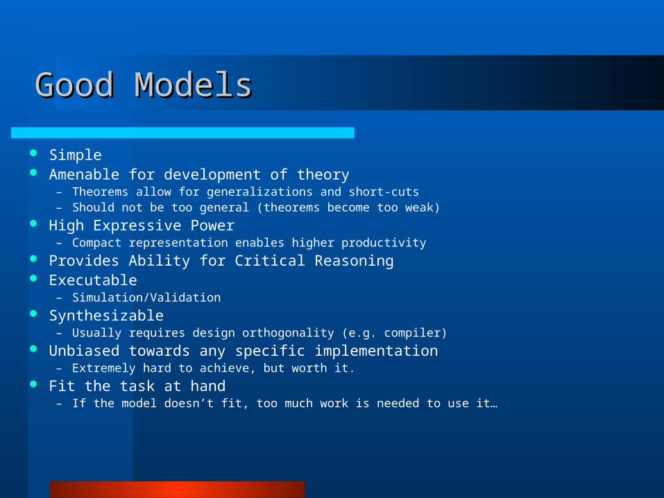
Good ModelsGood Models

Simple Amenable for development of theory

– Theorems allow for generalizations and short-cuts– Should not be too general (theorems become too weak)

High Expressive Power– Compact representation enables higher productivity

Provides Ability for Critical Reasoning Executable

– Simulation/Validation Synthesizable

– Usually requires design orthogonality (e.g. compiler) Unbiased towards any specific implementation

– Extremely hard to achieve, but worth it. Fit the task at hand

– If the model doesn’t fit, too much work is needed to use it…

Common Models of SystemsCommon Models of Systems

Finite State Machines/Regular Languages– finite state– full concurrency (notion of state)

Data-Flow/Process Models– Partial Order– Concurrent and sometimes Determinate– Stream of computation

Discrete-Event– Global Order (embedded in time)– Resolution Limits

Distributed-Event– Locally Discrete, Globally Asynchronous– Network Models

Continuous Time Simulation (Discrete Time Approx.)

– Spice (Matlab, Modelica)– Difference Equation analog of differential equations

of state

Frequency Domain– Harmonic Balance (Bode Plots)

Models fundamentally distinguished by how they model time

Notion of “State” is a fundamental abstraction (but is not reality)

All practical models have methods for attaining Coherent Behavior, event where synchronization cannot be achieved.

Model Of ComputationModel Of Computation

Requirement: A mathematical description of syntax and semantics. To be scalable, there are usually rules for model composition (support of hierarchy). To be practical, there are usually scope rules (support for abstraction and hiding). To be formally based, there needs to be unambiguous rules for forward propagation of time as well as a clear distinction of possible future states or paths.

Universe: A set of components (actors) and links (wires) with models for behavior within the semantics of the MOC and rules for composition of component behaviors into module behaviors. To enable synthesis or optimization we need a notion of module equivalence. To simplify analysis we need a set of invariants (global properties which always hold).

Metrics: A set of methods for assigning affine (ordered, comparable) parameters to modules, components, paths or other subsets to define quality measures or constraints. One can have parameter invariants as well.

Model Example: Spice (Circuit Simulator)Model Example: Spice (Circuit Simulator)

Continuous, parallel model of time• Resolution bounded by tolerance (defferential equation model)

Components are differential relations• Voltage change to Current (Capacitor)• Current change to Voltage (Inductor)• Sources (Voltage and Current)• State Dependent Devices (Transistors, TM-lines…)

Composition rules map voltages, conserve currents• Krichoff’s Laws (Model Invariants)

Support of Hierarchy, but not of abstraction• Subcircuits (replicate function, simple copying)

Only notion of equivalence is implied by .measure statements Tools for simulation of model, but not synthesis or formal analysis Useful despite model formal incompleteness

• Model is formally undecideable

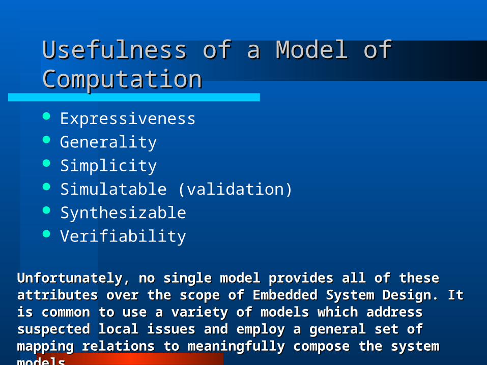
Usefulness of a Model of ComputationUsefulness of a Model of Computation

Expressiveness Generality Simplicity Simulatable (validation) Synthesizable Verifiability

Unfortunately, no single model provides all of these attributes over the scope of Unfortunately, no single model provides all of these attributes over the scope of Embedded System Design. It is common to use a variety of models which address Embedded System Design. It is common to use a variety of models which address suspected local issues and employ a general set of mapping relations to meaningfully suspected local issues and employ a general set of mapping relations to meaningfully compose the system models.compose the system models.

Simulation and SynthesisSimulation and Synthesis

Simulation: Prediction of future states or paths from a model given initial state(s) and span of time– Symbolic simulation: simulation where some fraction of the system

components are variables (unassigned models) Synthesis: Model refinement (construction of a particular module or

choice of and instance from a set with equivalent behaviors)– Must has notion of equivalence or at least containment– Often have metric for selection of instance

Verification: Proof of a formal property on a module over a set of possible activity traces (often simulation traces)– Exhaustive simulation– Symbolic exhaustive simulation

Validation: Assumption of a property by careful simulation of a model.– Coverage tools, Monte Carlo

Design/Component Validation TechniquesDesign/Component Validation Techniques

By construction– property is inherent.

By verification– property is provable.

By simulation– check behavior for all inputs.

By intuition– property is true. I just know it is.

By assertion/intimidation– property is true. Wanna make something of it?

Method of Ostrich– Don’t even try to doubt whether it is true

It is generally better to be higher in this list

Automated Specifications to Automated Specifications to Implementation (CAD/EDA/Compilers)Implementation (CAD/EDA/Compilers) Key Ideas: Abstraction, Model, Refinement, Composition,

Mapping, Binding, Design Metrics Given desired behavior, formulate satisfying model from abstract

component models using composition rules– System Behavior is a property of composition and of model

semantics– Composition rules describe how complex systems can be

assembled from isolated modules (hopefully enables metrics)– Semantics induced from composition rules and component behavior– Refinement describes an abstraction hierarchy with tree-like form

(rather than directed acyclic graph)– Mapping determines what subset of library instances are

functionally compatible with a given module– Binding is the process of selecting a particular instance of a less

abstract model from a library to replace a more abstract module

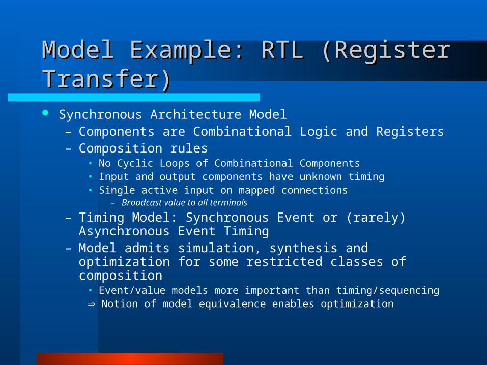
Model Example: RTL (Register Transfer)Model Example: RTL (Register Transfer)

Synchronous Architecture Model– Components are Combinational Logic and Registers– Composition rules

• No Cyclic Loops of Combinational Components• Input and output components have unknown timing• Single active input on mapped connections

– Broadcast value to all terminals

– Timing Model: Synchronous Event or (rarely) Asynchronous Event Timing

– Model admits simulation, synthesis and optimization for some restricted classes of composition

• Event/value models more important than timing/sequencing Notion of model equivalence enables optimization

Model Example: FSM (Finite Automata)Model Example: FSM (Finite Automata)

Components: “States” and “Transitions” Model Timing Behavior by series of “updates”

– Updates can be asynchronous on changing of inputs• Changing input changes states and potentially outputs

– Or can be synchronous on sampling clock• At each clock rising edge, examine inputs and determine if

transition can be made

Composition by Product– Possible states found by Cartesian Product of machines to

be composed– Model complexity grows very fast!

Supports Notions of Equivalence and Optimization

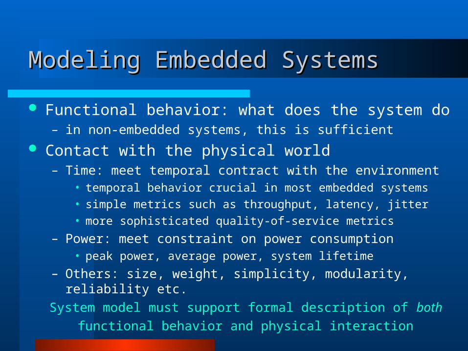
Modeling Embedded SystemsModeling Embedded Systems

Functional behavior: what does the system do– in non-embedded systems, this is sufficient

Contact with the physical world– Time: meet temporal contract with the environment

• temporal behavior crucial in most embedded systems

• simple metrics such as throughput, latency, jitter

• more sophisticated quality-of-service metrics

– Power: meet constraint on power consumption• peak power, average power, system lifetime

– Others: size, weight, simplicity, modularity, reliability etc.

System model must support formal description of both

functional behavior and physical interaction

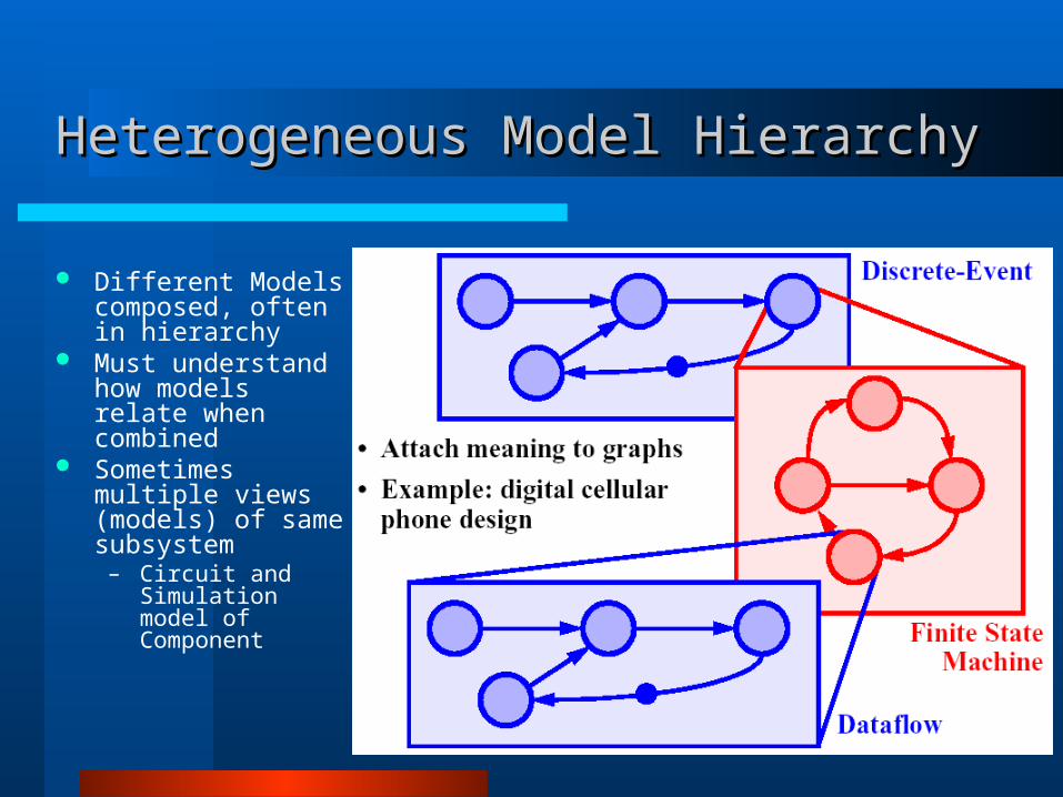
Heterogeneous Model HierarchyHeterogeneous Model Hierarchy

Different Models composed, often in hierarchy

Must understand how models relate when combined

Sometimes multiple views (models) of same subsystem

– Circuit and Simulation model of Component

““Textbook” SynthesisTextbook” Synthesis

Resources: 3 authors– Wrote 3 chapters each

Constraints:– Chapters Differ in

sizes/dependencies/topics

– Must cover “goal” chapter

– Must cover topic 7, but 8 is desirable

– Page limit (cost of book)

Chap Topics Requires Pages

A 1,3 - 48

B 2,3 - 55

C 1,4 2 39

D 2 - 33

E 3,5 1,4 42

F 6 3,2 60

G 7* 3,4,5 32

H 6,8 1,5 58

I 7* 2,3 71

““Textbook” SynthesisTextbook” Synthesis

Chap Topics Requires Pages

A 1,3 - 48

B 2,3 - 55

C 1,4 2 39

D 2 - 33

E 3,5 1,4 42

F 6 3,2 60

G 7* 3,4,5 32

H 6,8 1,5 58

I 7* 2,3 71

A48

I71

H58

G32

F60

E42

D33

C39

B55

““Textbook” SynthesisTextbook” Synthesis

DCEG supplants BCEG Cheapest “Cover” =204 Publisher might choose both

DCEG and BFI… Page cost constraint propagated

from chapters to book

Soln Topics Pages

B,I 2,3,7 126

D,C,E,G 1,2,3,4,5,7 146

D,C,E,G,H All 204

B,F,I 2,3,6,7 186

B,C,E,G 1,2,3,4,5,7 168

A48

I71

H58

G32

F60

E42

D33

C39

B55

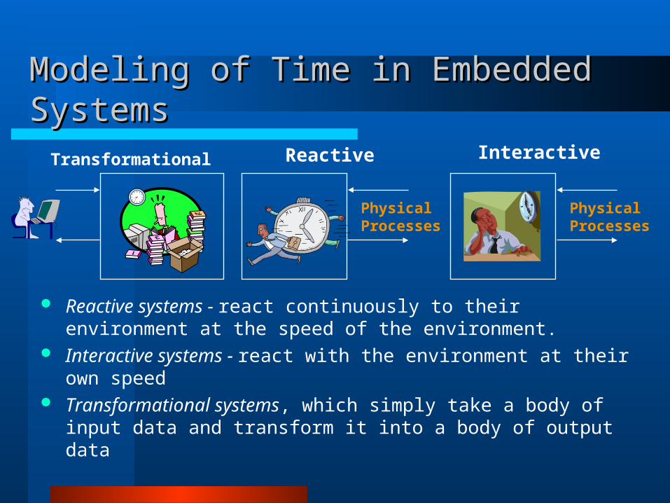
Modeling of Time in Embedded SystemsModeling of Time in Embedded Systems

Reactive systems - react continuously to their environment at the speed of the environment.

Interactive systems - react with the environment at their own speed Transformational systems, which simply take a body of input data

and transform it into a body of output data

Transformational Reactive Interactive

PhysicalProcesses

PhysicalProcesses

Importance of Time in Embedded Systems: Importance of Time in Embedded Systems: Reactive OperationReactive Operation

Computation is in response to external events– periodic events can be statically scheduled

– aperiodic events tricky to analyze• Worst-case is over-design• statistically predict and dynamically schedule• approximate computation algorithms

As opposed to Transformation or Interactive Systems– Typically care about throughput, bandwidth, capacity

– (Typical performance metrics for classical computation)

A ‘faster’ computer might be more reactive – but might not– Issue: Latency versus Throughput

Reactive OperationReactive Operation

Interaction with environment causes problems– indeterminacy in execution

• e.g. waiting for events from multiple sources

– physical environment is delay intolerant• can’t put it on wait with an hour glass icon!

Handling timing constraints are crucial to the design of embedded systems– interface synthesis, scheduling etc.– increasingly, also implies high performance– Correctness implies timely response!

In many time-critical applications, processor caches are disabled to simplify system timing verification

Shades of Real-timeShades of Real-time

Hard– the right results late are wrong!– catastrophic failure if deadline not met– safety-critical

Soft– the right results late are of less value than right results on time

• more they are late, less the value, but do not constitute system failure• usually average case performance is important

– failure not catastrophic, but impacts service quality• e.g. connection timing out, display update in games

– most systems are largely soft real-time with a few hard real-time constraints (End-to-end) quality of service (QoS)

– notion from multimedia/OS/networking area– encompasses more than just timing constraints– classical real-time is a special case

Many Notions of TimeMany Notions of Time

How do the models differ?How do the models differ?

State: finite vs. infinite Time: untimed, continuous time, partial order, global order Concurrency: sequential, concurrent Determinacy: determinate vs. indeterminate Data value: continuous, sample stream, event Communication mechanisms Others: composition, availability of tools etc.

How to apply this?How to apply this?

Models are all well and good– But need to get heads out of clouds and write software

Examine Classical Application– Simple Real-time system– See how/where models apply– How can we use these ideas to make simpler, more reliable

design?

Software Timing:– Modules take some number of processor cycles– Often input data or size dependent– Typical model: T(total) = Throughput * Size + Setup– Timings subject to hardware overhead and conflicts

Deterministic Real-Time ProgrammingDeterministic Real-Time Programming

Processor activity mediated by Clock– 5MHz-1+Ghz– Instruction timing scaled by small number of clocks

Simplest reactive system: “Grand Loop”– All desired system behaviors can be addressed in similar

time scales– Relatively few desired behaviors (else excessive loop

latency)– Initialization and error recovery must also be captured in

loop behavior

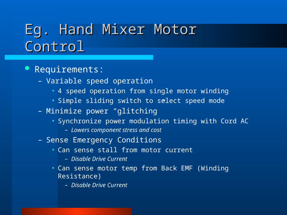
Eg. Hand Mixer Motor ControlEg. Hand Mixer Motor Control

Requirements:– Variable speed operation

• 4 speed operation from single motor winding

• Simple sliding switch to select speed mode

– Minimize power “glitching”• Synchronize power modulation timing with Cord AC

– Lowers component stress and cost

– Sense Emergency Conditions• Can sense stall from motor current

– Disable Drive Current

• Can sense motor temp from Back EMF (Winding Resistance)– Disable Drive Current

Hand Mixer Control IIHand Mixer Control II

Strategy:– Build simple looping program:

• Timing of loop is bounded– Add no-ops if loop runs too fast

• Behaviors can all be setup to run incrementally– Small number of instructions for each “task”

• Initialization and reset can be made implicit

– Low cost, low complexity

Mixer Control LoopMixer Control Loop

“Sample” inputs each cycle– Power AC level

– Switch State

– Back EMF of Windings• level allows measurement of motor speed)

Update Internal “state”– Motor Temp, Speed, Acceleration, Mode (Desired Speed)

Check for Conditions– Mode Change; Load, Temp bounds; Initialization (power on)

Outputs each cycle– Drive On/Off (Often Pulse-Mode, often synchronized with AC power

– Indicator Lights (power-on, overload, temperature warning)

Mixer Program IssuesMixer Program Issues

Loop needs to be fast, but not too fast– “fast” means several-many loops of code per system event

timescales– Power cycles 60Hz => 16.667mS, 1% of cycle = 1V =>

166uS max– Motor Drive Frequency Response

• Do not wish to excite vibration resonance of mechanical parts• Too-slow or Harmonic: motor “singing” or “hum”• Too-fast: Switching time of drive (few uS) happens so often that

switching losses (heat!) increases cost and complexity of motor drive circuitry

Eg. 10MHz PIC (~2.5M ins/Sec) get 2.5*166 = 416 instructions max in loop, 800 in 20MHz version

Issues in “Grand Loop”Issues in “Grand Loop”

Requires ability to “free-run” system– Needs predictable loop timing => Fixed instruction execution latency

• Caches, Conditional Hazards etc. will cause timing jitter

– Can handle low frequency behaviors to a limited degree• Counters can create long-term event management• Measurement of slow events limited by sampling noise

– Processor Runs at all times• Not a great low-power solution (i.e. Hearing aid)

Such Systems are called “Polled Operation”– Very cheap and popular, very reliable, simple and easy to

debug

Higher Precision (maybe) Timed EventsHigher Precision (maybe) Timed Events

Problem: Some systems have random timed events which cause modal changes to behavior or have control loops which are too long to execute completely between samples or maybe samples must be asynchronous– Eg Powerswitch, trash can lid opener, Chromatic tuner

Idea: Divide behaviors into long-term and short-term– Make use of built-in hardware (interrupts)– Long-term code can still run in loop – – But short-term events handled in asynchronous interrupt

routines

Interrupt based Program ControlInterrupt based Program Control

Advantages:– Short time to service event compared to worst-case polling– Can use event timing to loosely synchronize program behavior, even

if instruction throughput is not very constant– Some architectures allow for low-power execution while awaiting

interrupts Issues:

– Breaks program control flow model• Special programming requirements• Difficult to debug since bugs may require complex temporal conditions

– Architecture Specific Program Accommodations • Stack Conventions, Dynamic Program Status, Semaphores and access

arbitration• Assembly Language “Drop-ins”, Function Attributes• Compiler Optimization and code generation

Faster than Interrupts?Faster than Interrupts?

Hardware Appliances:– The Ubiquitous Timer

• 16/32/64 bit, often small multiple of clock tick• Often provides for Interrupt sourcing• Polled to provide reference clock time

– Timed Sampler/PWM or Sigma-Delta Actuator• Hardware timed circuit with jitter levels in pS.• Often Fifo buffer to connect to software• Common Scheme for medium/high performance signal conversion

– DMA Controller• Simple bus driver with fixed, high performance timing• Provides data loading, sometimes in parallel with program execution

Program Timed Behavior ConclusionsProgram Timed Behavior Conclusions

Complexity of Solution is a direct function of– Relative timescale of Behaviors– Absolution timescale of sampling and actuation– Complexity of Desired Response

Need to minimize number of architecture specific interventions

Polling vs. Interrupts vs. Hardware Modules– Issue is often worst case latency between event and

response

SparesSpares

Real Time OperationReal Time Operation

Correctness of result is a function of time it is delivered: the right results on time!– deadline to finish computation– doesn’t necessarily mean fast: predictability is important– worst case performance is often the issue

• but don’t want to be too pessimistic (and costly)

Accurate performance prediction needed

++

D1

++

x y

D2Longest Path for TSTS = m + 2

Longest Path for TLTL = 2m + 3

Achievable Latency: Pipeline ModuleAchievable Latency: Pipeline Module

Common trick to improve performance at cost of storage:– Introduce storage in intermediate computation stages– Enables new computations to start before prior computations are

completed (very common practice in hardware design)– Leads to improved throughput by reusing hardware components

but has power and total latency cost

Timing ConstraintsTiming Constraints

Timing constraints are the key feature!• impose temporal restrictions on a system or its users

• hard timing constraints, soft timing constraints, interactive

Questions:• What kind of timing constraints are there?

• How do we arrange computation to take place such that it satisfies the timing constraints?

Timing Models used for Embedded SystemsTiming Models used for Embedded Systems

Finite State Machines Communicating Finite State Machines Discrete Event Synchronous / Reactive Dataflow Process Networks Rendezvous-based Models (CSP) Petri Nets Tagged-Signal Model

RTL Node Retiming (Optimization)RTL Node Retiming (Optimization)

For RTL model add the following:1. Inputs/Outputs are synchronized2. Equivalence of Models means identical input and output

sequences3. Minimize Clock timing (minimize maximum timing path

between registers) (Optimization Metric)4. All registers assigned along links

Can formulate algorithm for any legal RTL model to assign registers such that behavior is equivalent to initial assignment and metric is minimized

– Node retiming does not alter topology of dataflow, just timing of activities

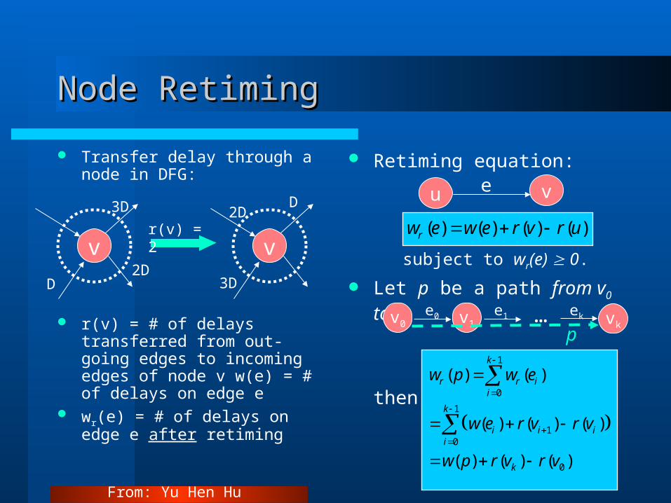
Retiming equation:

subject to wr(e) 0.

Let p be a path from v0 to vk

then

Node RetimingNode Retiming

Transfer delay through a node in DFG:

r(v) = # of delays transferred from out-going edges to incoming edges of node v w(e) = # of delays on edge e

wr(e) = # of delays on edge e after retiming

v v

3D

D2D

3D

D2D

r(v) = 2 ( ) ( ) ( ) ( )rw e w e r v r u

1

0

1

10

0

( ) ( )

( ) ( ) ( )

( ) ( ) ( )

k

r r ii

k

i i ii

k

w p w e

w e r v r v

w p r v r v

v0e0 v1

e1 … vkek

u ve

p

From: Yu Hen Hu 2006

DFG ExampleDFG Example

T = max. {(1+2+1)/2, (1+2+1)/3} = 2Max Path delay = 2+1 = 3

T = max. {(1+2+1)/2, (1+2+1)/3} = 2Max Path Delay = max{2,2,1+1} = 2

From: Yu Hen Hu 2006

Systematic SolutionsSystematic Solutions

Given a systems of inequalities:

r(i) – r(j) k; 1 i,j N

Construct a constraint graph:1. Map each r(i) to node i. Add

a node N+1.

2. For each inequality

r(i) – r(j) k,

draw an edge eji

such that w(eji) = k.

1. Draw N edges eN+1,i = 0.

a) The system of inequalities has a solution if and only if the constraint graph contains no negative cycles

b) If a solution exists, one solution is where ri is the minimum length path from the node N+1 to the node i.

Shortest path algorithms:Bellman-Ford algorithm

Floyd-Warshall algorithm

From: Yu Hen Hu 2006

Floyd-Warshall AlgorithmFloyd-Warshall Algorithm

Find shortest path between all possible pairs of nodes in the graph provided no negative cycle exists.

Algorithm:

Initialization: R(1) =W;

For k=1 to N R(k+1)(u,v) = min{R(k)(u,:) + R(k)(:,v)}

If R(k)(u,u) < 0 for any k, u, then a negative cycle exists.

Else, R(N+1)(u,v) is SP from u to v

21

34

21

2

3

1

(2)

(3) (4) (5)

0 3 0 3 2 1

0 1 2 3 0 1 2

0 2 3 0 2

1 0 1 2 0

0 3 2 1

3 0 1 2

3 0 0 2

1 2 1 0

W R

R R R

From: Yu Hen Hu 2006

More General Timing ConstraintsMore General Timing Constraints

Two categories of timing constraints– Performance constraints: set limits on response time of the system– Behavioral constraints: make demand on the rate at which users supply

stimuli to the system Further classification: three types of temporal restrictions (not mutually

exclusive)– Maximum: no more than t amount of time may elapse between the occurrence of

one event and the occurrence of another– Minimum: No less than t amount of time may elapse between two events– Durational: an event must occur for t amount of time

Note: “Event” is either a stimulus to the system from its environment, or is an externally observable response that the system makes to its environment

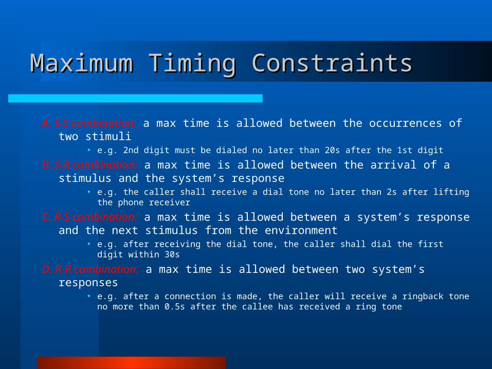
Maximum Timing ConstraintsMaximum Timing Constraints

A. S-S combination: a max time is allowed between the occurrences of two stimuli

• e.g. 2nd digit must be dialed no later than 20s after the 1st digit

B. S-R combination: a max time is allowed between the arrival of a stimulus and the system’s response

• e.g. the caller shall receive a dial tone no later than 2s after lifting the phone receiver

C. R-S combination: a max time is allowed between a system’s response and the next stimulus from the environment

• e.g. after receiving the dial tone, the caller shall dial the first digit within 30s

D. R-R combination: a max time is allowed between two system’s responses• e.g. after a connection is made, the caller will receive a ringback tone no more than

0.5s after the callee has received a ring tone

Control Flow versus Data FlowControl Flow versus Data Flow

Fuzzy distinction, yet useful for:– specification (language, model, ...)– synthesis (scheduling, optimization, ...)– validation (simulation, formal verification, ...)

Roughly:– control:

• Small number of possible values• don’t know when data arrives (quick reaction)• time of arrival often matters more than value

– data:• Large number of possible values• data arrives in regular streams (samples)• value matters most

Control versus Data FlowControl versus Data Flow

Specification, synthesis and validation methods emphasize:–for control:

• event/reaction relation• response time

–Real Time scheduling to meet deadlines

• priority among events and processes

–for data:• functional dependency between input and output• memory/time efficiency

–Dataflow scheduling for efficient execution

• all events and processes are equal–Throughput is usual goal

To Speculate or not…To Speculate or not…

A fundamental trick common to many levels of architecture is average throughput improvement by speculation

– Branch speculation improves performance based on guessing program flow• Cheap to support since limited number of futures

• (Control speculation)

– A cache operates by speculating on future data access locality• Many futures, but can be systematic, usually waits on miss (P4 did replay instead)

• (Data Speculation)

– Both tricks have software analogs despite serial nature of code

• Many software algorithms devolve to specialized search

Speculation tradeoffs are based on performance versus overhead (storage and time costs)

– Can be automated given systematic Models and Metrics

Rarely helps latency, but helps latency at higher levels of abstraction