Lecture 2: Bayesian Hypothesis Testing - CBMS-MUM · ’CBMS: Model Uncertainty and Multiplicity...

CBMS: Model Uncertainty and Multiplicity Santa Cruz, July 23-28, 2012'

&

$

%

Lecture 2: Bayesian Hypothesis Testing

Jim Berger

Duke University

CBMS Conference on Model Uncertainty and MultiplicityJuly 23-28, 2012

1


&

$

%

Outline

• Pedagogical introduction to Bayesian testing

• Formal introduction to Bayesian testing

• Precise and imprecise hypotheses

• Choice of prior distributions for testing

• Paradoxes

• Robust Bayesian testing

• Multiple hypotheses and sequential testing

• HIV vaccine example

• Psychokinesis example

• More on p-values and their calibration

2


&

$

%

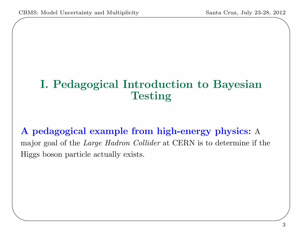
I. Pedagogical Introduction to BayesianTesting

A pedagogical example from high-energy physics: A

major goal of the Large Hadron Collider at CERN is to determine if the

Higgs boson particle actually exists.

3


&

$

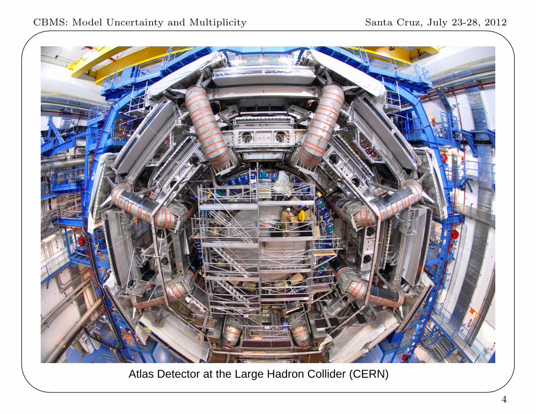
%Atlas Detector at the Large Hadron Collider (CERN)

4


&

$

%

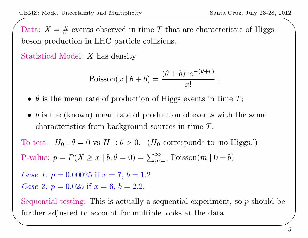
Data: X = # events observed in time T that are characteristic of Higgs

boson production in LHC particle collisions.

Statistical Model: X has density

Poisson(x | θ + b) =(θ + b)xe−(θ+b)

x!;

• θ is the mean rate of production of Higgs events in time T ;

• b is the (known) mean rate of production of events with the same

characteristics from background sources in time T .

To test: H0 : θ = 0 vs H1 : θ > 0. (H0 corresponds to ‘no Higgs.’)

P-value: p = P (X ≥ x | b, θ = 0) =∑∞

m=x Poisson(m | 0 + b)

Case 1: p = 0.00025 if x = 7, b = 1.2

Case 2: p = 0.025 if x = 6, b = 2.2.

Sequential testing: This is actually a sequential experiment, so p should be

further adjusted to account for multiple looks at the data.

5


&

$

%

Bayes factor of H0 to H1: ratio of likelihood under H0 to average likelihood

under H1 (or “odds” of H0 to H1)

B01(x) =Poisson(x | 0 + b)∫∞

0Poisson(x | θ + b)π(θ) dθ

=bx e−b∫∞

0(θ + b)x e−(θ+b)π(θ) dθ

.

Subjective approach: Choose π(θ) subjectively (e.g., using the standard

physics model predictions of the mass of the Higgs).

Objective approach: Choose π(θ) to be the ‘intrinsic prior’ (discussed later)

πI(θ) = b(θ + b)−2. (Note that this prior is proper and has median b.)

Bayes factor: is then given by

B01 =bx e−b∫∞

0(θ + b)x e−(θ+b)b(θ + b)−2 dθ

=b(x−1) e−b

Γ(x− 1, b),

where Γ is the incomplete gamma function.

Case 1: B01 = 0.0075 (recall p = 0.00025)

Case 2: B01 = 0.26 (recall p = 0.025)

6


&

$

%

Posterior probability of the null hypothesis: The objective choice of prior

probabilities of the hypotheses is Pr(H0) = Pr(H1) = 0.5, in which case

Pr(H0 | x) = B01

1 +B01.

Case 1: Pr(H0 | x) = 0.0075 (recall p = 0.00025)

Case 2: Pr(H0 | x) = 0.21 (recall p = 0.025)

Complete posterior distribution: is given by

• Pr(H0 | x), the posterior probability of null hypothesis

• π(θ | x,H1), the posterior distribution of θ under H1

A useful summary of the complete posterior is Pr(H0 | x) andC, a (say) 95% posterior credible set for θ under H1.

Case 1: Pr(H0 | x) = 0.0075; C = (1.0, 10.5)

Case 2: Pr(H0 | x) = 0.21; C = (0.2, 8.2)

Note: For testing precise hypotheses, confidence intervals alone are not a

satisfactory inferential summary.

7


&

$

%

0 2 4 6 8 10 12

0.00

0.05

0.10

0.15

0.0075

Figure 1: Pr(H0 | x) (the vertical bar), and the posterior density for θ given

x and H1.

8


&

$

%

What should a Fisherian or a frequentist think of thediscrepancy between the p-value and the objective Bayesiananswers in precise hypothesis testing?

Many Fisherians (and arguably Fisher) prefer likelihood ratios to p-values,

when they are available (e.g., genetics).

A lower bound on the Bayes factor (or likelihood ratio): choose π(θ) to be

a point mass at θ, yielding

B01(x) =Poisson(x | 0 + b)∫∞

0Poisson(x | θ + b)π(θ) dθ

≥ Poisson(x | 0 + b)

Poisson(x | θ + b)= min{1,

(b

x

)x

ex−b} .

Case 1: B01 ≥ 0.0014 (recall p = 0.00025)

Case 2: B01 ≥ 0.11 (recall p = 0.025)

Note: Such arguments were first used in

Edwards, W., Lindman, H., and Savage, L. J. (1963), “Bayesian Statistical

Inference for Psychological Research,” Psychological Review, 70,193-242.

9


&

$

%

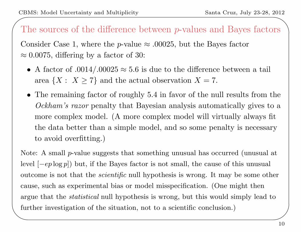
The sources of the difference between p-values and Bayes factors

Consider Case 1, where the p-value ≈ .00025, but the Bayes factor

≈ 0.0075, differing by a factor of 30:

• A factor of .0014/.00025 ≈ 5.6 is due to the difference between a tail

area {X : X ≥ 7} and the actual observation X = 7.

• The remaining factor of roughly 5.4 in favor of the null results from the

Ockham’s razor penalty that Bayesian analysis automatically gives to a

more complex model. (A more complex model will virtually always fit

the data better than a simple model, and so some penalty is necessary

to avoid overfitting.)

Note: A small p-value suggests that something unusual has occurred (unusual at

level [−ep log p]) but, if the Bayes factor is not small, the cause of this unusual

outcome is not that the scientific null hypothesis is wrong. It may be some other

cause, such as experimental bias or model misspecification. (One might then

argue that the statistical null hypothesis is wrong, but this would simply lead to

further investigation of the situation, not to a scientific conclusion.)

10


&

$

%

II. Formal Introduction to Bayesian Testing

11


&

$

%

Notation

• X | θ ∼ f(x | θ).

• To test: H0 : θ ∈ Θ0 vs H1 : θ ∈ Θ1 .

• Prior distribution:

– Prior probabilities Pr(H0) and Pr(H1) of the hypotheses.

– Proper prior densities π0(θ) and π1(θ) on Θ0 and Θ1.

∗ πi(θ) would be a point mass if Θi is a point.

• Marginal likelihoods under the hypotheses:

m(x | Hi) =

∫Θi

f(x | θ)πi(θ) dθ, i = 0, 1 .

• Bayes factor of H0 to H1:

B01 =m(x | H0)

m(x | H1).

12


&

$

%

Conclusions from posterior probabilities or Bayes factors:

• Based on the posterior odds. By default, H0 accepted if

Pr(H0 | x) > Pr(H1 | x) but often decisions are not reported.

• Alternatively, report Bayes factor B01 either because

– it is to be combined with personal prior odds

– the ‘default’ Pr(H0) = Pr(H1) is used.

– Jeffreys (1961) suggested the scale

B01 Strength of evidence

1:1 to 3:1 Barely worth mentioning

3:1 to 10:1 Substantial

10:1 to 30:1 Strong

30:1 to 100:1 Very strong

> 100:1 Decisive

14


&

$

%

• More generally, use a 0−Ki loss function:

L(θ, ai) =

0, if θ ∈ Θi

Ki, if θ ∈ Θj , j = i

• Optimal decision a1 (reject H0) iif

Pr(H0 | x)Pr(H1 | x)

<K0

K1.

• Bayesian rejection regions are usually of same form as classical

rejection regions but (fixed) cut-off points are determined by loss

functions and prior odds.

16


&

$

%

III. Precise and Imprecise Hypotheses

(Point Null and One-Sided Hypotheses)

17


&

$

%

A Key Issue: Is the precise hypothesis being tested plausible?

A precise hypothesis is an hypothesis of lower dimension than the

alternative (e.g. H0 : µ = 0 versus H0 : µ = 0).

A precise hypothesis is plausible if it has a reasonable prior probability of

being true. H0 : there is no Higgs boson particle, is plausible.

Example: Let θ denote the difference in mean treatment effects for cancer

treatments A and B, and test H0 : θ = 0 versus H1 : θ = 0.

Scenario 1: Treatment A = standard chemotherapy

Treatment B = standard chemotherapy + steroids

Scenario 2: Treatment A = standard chemotherapy

Treatment B = a new radiation therapy

H0 : θ = 0 is plausible in Scenario 1, but not in Scenario 2; in the latter

case, instead test H0 : θ < 0 versus H1 : θ > 0.

18


&

$

%

Plausible precise null hypotheses:

• H0 : Males and females of a species have the same characteristic A.

• H0 : Pollutant A does not affect Species B.

• H0 : Gene A is not associated with Disease B.

• H0: There is no psychokinetic effect.

• H0: Vitamin C has no effect on the common cold.

• H0: A new HIV vaccine has no effect.

• H0: Cosmic microwave background radiation is isotropic.

Implausible precise null hypotheses:

• H0 : Small mammals are as abundant on livestock grazing land as on

non-grazing land

• H0 : Bird abundance does not depend on the type of forest habitat

they occupy

• H0 : Children of different ages react the same to a given stimulus.

19


&

$

%

An Aside: Hypothesis Testing is Drastically Overused

• Tests are often performed when they are irrelevant.

• Rejection by an irrelevant test is sometimes viewed as “license” to

forget statistics in further analysis

A wildlife example:

Habitat Rank Observed

Type Usage Hypothesis

A 1 3.8

B 2 3.6 H0: “mean usage of habitats by a type

C 3 2.8 of bird is equal for all habitats ”

D 4 1.8 Rejected (p < .025)

E 5 1.5

F 6 0.7

20


&

$

%

Statistical mistakes in the example

• The hypothesis is not plausible; testing serves no purpose.

• The observed usage levels are given without confidence sets.

• The rankings are based only on observed means, and are given without

uncertainties. (For instance, suppose a 95% confidence interval for A is

(1.8,5.8), while that for B is (3.5,3.7).)

21


&

$

%

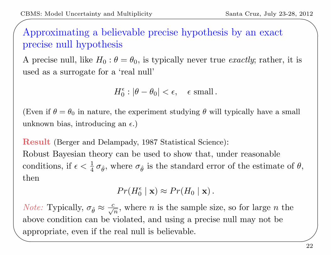
Approximating a believable precise hypothesis by an exactprecise null hypothesis

A precise null, like H0 : θ = θ0, is typically never true exactly; rather, it is

used as a surrogate for a ‘real null’

Hϵ0 : |θ − θ0| < ϵ, ϵ small .

(Even if θ = θ0 in nature, the experiment studying θ will typically have a small

unknown bias, introducing an ϵ.)

Result (Berger and Delampady, 1987 Statistical Science):

Robust Bayesian theory can be used to show that, under reasonable

conditions, if ϵ < 14 σθ, where σθ is the standard error of the estimate of θ,

then

Pr(Hϵ0 | x) ≈ Pr(H0 | x) .

Note: Typically, σθ ≈ c√n, where n is the sample size, so for large n the

above condition can be violated, and using a precise null may not be

appropriate, even if the real null is believable.

22


&

$

%

Posterior probabilities can equal p-values in one-sided testing:

Normal Example:

• X | θ ∼ N(x | θ, σ2)

• One-sided testing

H0 : θ ≤ θ0 vs H1 : θ > θ0

• Choose the usual estimation objective prior π(θ) = c, yielding posterior

θ | x ∼ N(θ | x, σ2).

• Posterior probability of H0:

Pr(H0 | x) = Pr(θ ≤ θ0 | x) = Φ

(θ0 − x

σ

)= 1− Φ

(x− θ0

σ

)= Pr(X > x | θ0) = p-value .

23


&

$

%

• The Bayes factor can also be formally defined as

B01 =

∫ θ0−∞ N(x | θ, σ)c dθ∫∞θ0

N(x | θ, σ)c dθ=

Φ((θ0 − x)/σ)

1− Φ((θ0 − x)/σ),

since the unspecified constant c in the Bayes factor cancels.

– This can be rigorously justified as resulting from a limit of vague

proper priors symmetric about θ0.

• If, instead, one were testing

H0 : 0 ≤ θ ≤ θ0 vs H1 : θ > θ0 ,

use of π(θ) = c is much more problematical (in that one appears to be

giving infinite prior odds in favor of H1).

• It has been argued (e.g., Berger and Mortera, JASA99) that objective

testing in one-sided cases should not use objective estimation priors.

24


&

$

%

IV. Choice of Prior Distributions in Testing

25


&

$

%

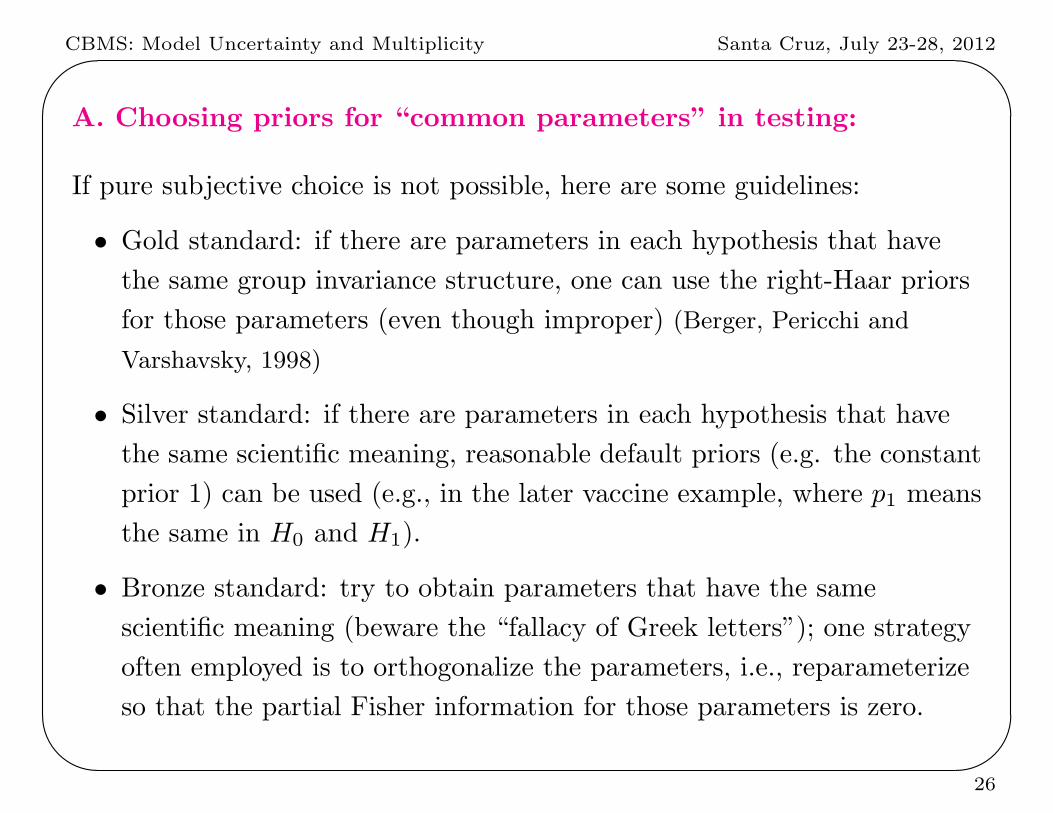
A. Choosing priors for “common parameters” in testing:

If pure subjective choice is not possible, here are some guidelines:

• Gold standard: if there are parameters in each hypothesis that have

the same group invariance structure, one can use the right-Haar priors

for those parameters (even though improper) (Berger, Pericchi and

Varshavsky, 1998)

• Silver standard: if there are parameters in each hypothesis that have

the same scientific meaning, reasonable default priors (e.g. the constant

prior 1) can be used (e.g., in the later vaccine example, where p1 means

the same in H0 and H1).

• Bronze standard: try to obtain parameters that have the same

scientific meaning (beware the “fallacy of Greek letters”); one strategy

often employed is to orthogonalize the parameters, i.e., reparameterize

so that the partial Fisher information for those parameters is zero.

26


&

$

%

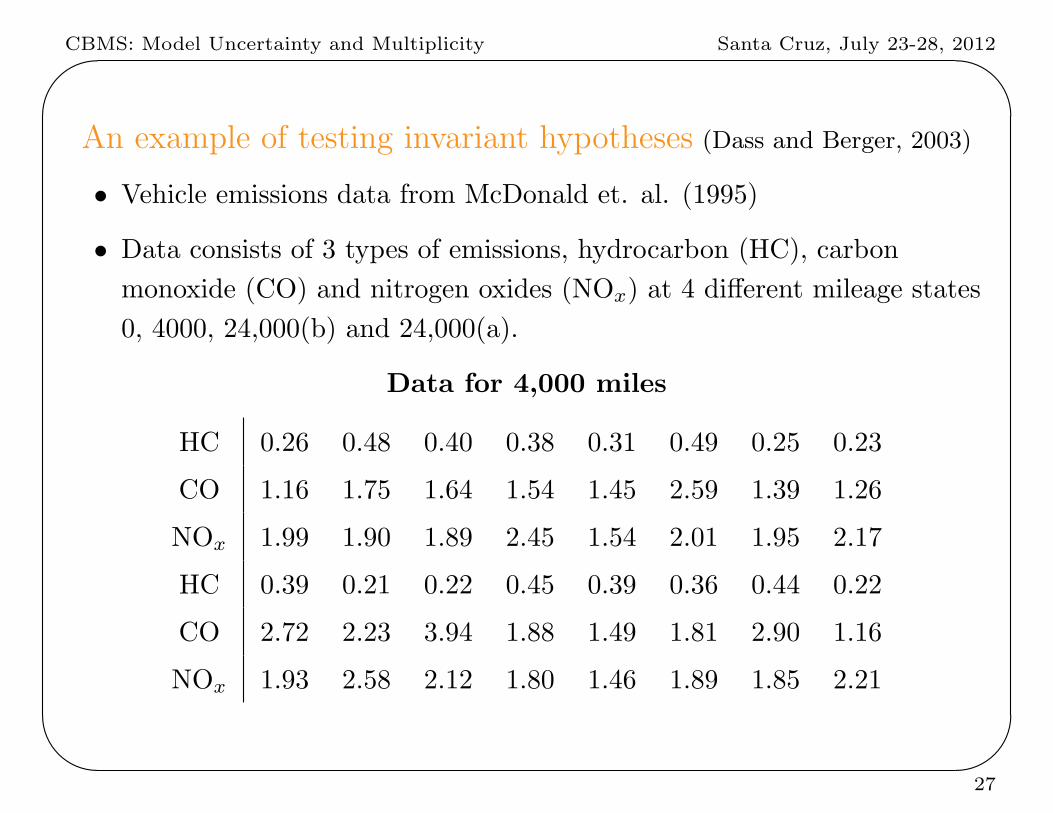
An example of testing invariant hypotheses (Dass and Berger, 2003)

• Vehicle emissions data from McDonald et. al. (1995)

• Data consists of 3 types of emissions, hydrocarbon (HC), carbon

monoxide (CO) and nitrogen oxides (NOx) at 4 different mileage states

0, 4000, 24,000(b) and 24,000(a).

Data for 4,000 miles

HC 0.26 0.48 0.40 0.38 0.31 0.49 0.25 0.23

CO 1.16 1.75 1.64 1.54 1.45 2.59 1.39 1.26

NOx 1.99 1.90 1.89 2.45 1.54 2.01 1.95 2.17

HC 0.39 0.21 0.22 0.45 0.39 0.36 0.44 0.22

CO 2.72 2.23 3.94 1.88 1.49 1.81 2.90 1.16

NOx 1.93 2.58 2.12 1.80 1.46 1.89 1.85 2.21

27


&

$

%

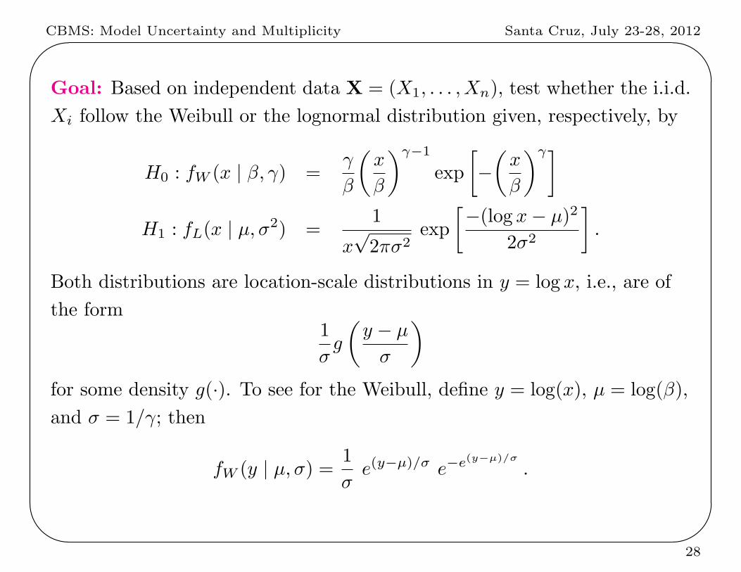
Goal: Based on independent data X = (X1, . . . , Xn), test whether the i.i.d.

Xi follow the Weibull or the lognormal distribution given, respectively, by

H0 : fW (x | β, γ) =γ

β

(x

β

)γ−1

exp

[−(x

β

)γ]H1 : fL(x | µ, σ2) =

1

x√2πσ2

exp

[−(log x− µ)2

2σ2

].

Both distributions are location-scale distributions in y = log x, i.e., are of

the form1

σg

(y − µ

σ

)for some density g(·). To see for the Weibull, define y = log(x), µ = log(β),

and σ = 1/γ; then

fW (y | µ, σ) = 1

σe(y−µ)/σ e−e(y−µ)/σ

.

28


&

$

%

Berger, Pericchi and Varshavsky (1998) argue that, for two hypotheses

(models) with the same invariance structure (here location-scale

invariance), one can use the right-Haar prior (usually improper) for both.

Here the right-Haar prior is

πRH(µ, σ) =1

σdσdµ .

The justification is called predictive matching and goes as follows (related

to arguments in Jeffreys 1961):

• With only two observations (y1, y2), one cannot possibly distinguish

between fW (y | µ, σ) and fL(y | µ, σ) so we should have B01(y1, y2) = 1.

• Lemma:∫ ∞

0

∫ ∞

−∞

1

σg

(y1 − µ

σ

)1

σg

(y2 − µ

σ

)πRH(µ, σ)dµdσ =

1

2|y1 − y2|

for any density g(·), implying B01(y1, y2) = 1 for two location-scale

densities.

29


&

$

%

Using the right-Haar prior for both models, calculus then yields that Bayes

factor of H0 to H1 is

B(X) =Γ(n)nnπ(n−1)/2

Γ(n− 1/2)

∫ ∞

0

[v

n

n∑i=1

exp

(yi − y

syv

)]−n

dv,

where y = 1n

∑ni=1 yi and s2y = 1

n

∑ni=1(yi − y)2. Note: This is also the

classical UMP invariant test statistic.

As an example, consider four of the car emission data sets, each giving the

carbon monoxide emission at a different mileage level.

For testing, H0 : Lognormal versus H1 : Weibull, the results were as

follows:

Data set at Mileage level

0 4000 24,000 30,000

B01 0.404 0.110 0.161 0.410

30


&

$

%

Dass and Berger (2003) showed that this is also a situation where

conditional frequentist testing, using the p-value conditioning statistic, can

be done resulting in the test:

TB =

if B(x) ≤ 0.94, reject H0, report Type I CEP

α(x) = B(x)/(1 +B(x)) ;

if B(x) > 0.94, accept H0, report Type II CEP

β(x) = 1/(1 +B(x)).

Note: The CEPs are the same for any value of the parameters under the

models (because of invariance) and again equal the objective Bayesian

posterior probabilities of the hypotheses.

31


&

$

%

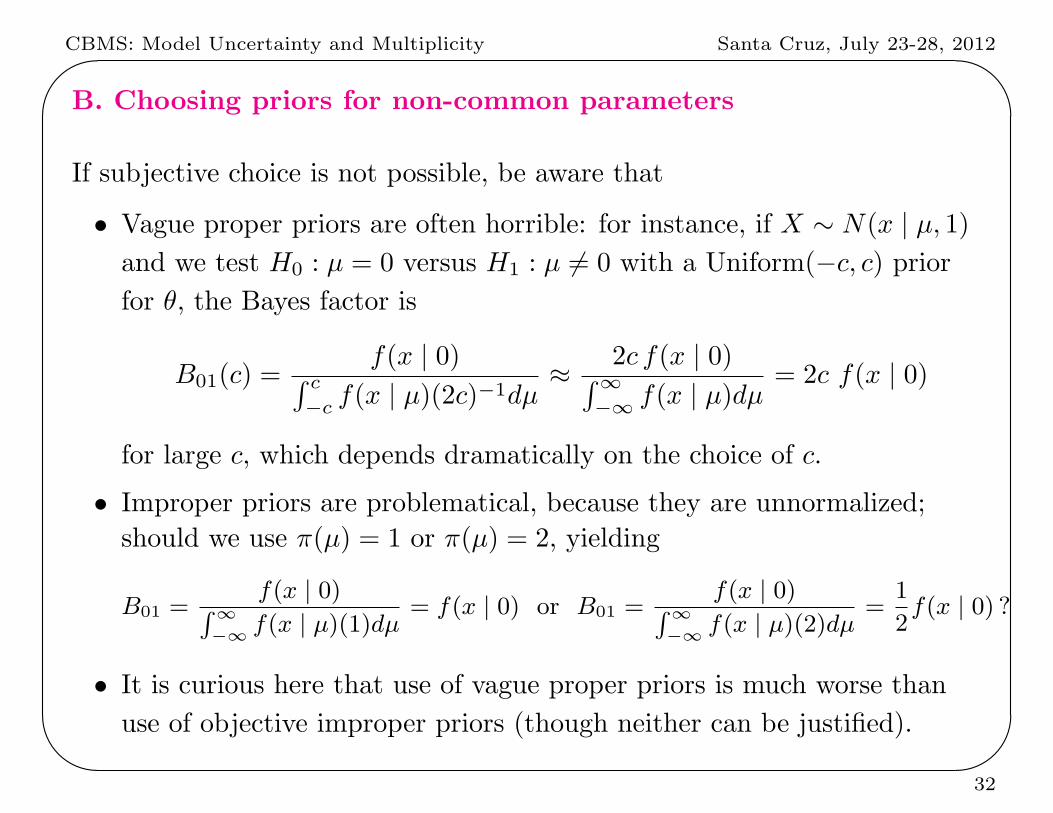
B. Choosing priors for non-common parameters

If subjective choice is not possible, be aware that

• Vague proper priors are often horrible: for instance, if X ∼ N(x | µ, 1)and we test H0 : µ = 0 versus H1 : µ = 0 with a Uniform(−c, c) prior

for θ, the Bayes factor is

B01(c) =f(x | 0)∫ c

−cf(x | µ)(2c)−1dµ

≈ 2c f(x | 0)∫∞−∞ f(x | µ)dµ

= 2c f(x | 0)

for large c, which depends dramatically on the choice of c.

• Improper priors are problematical, because they are unnormalized;

should we use π(µ) = 1 or π(µ) = 2, yielding

B01 =f(x | 0)∫∞

−∞ f(x | µ)(1)dµ= f(x | 0) or B01 =

f(x | 0)∫∞−∞ f(x | µ)(2)dµ

=1

2f(x | 0) ?

• It is curious here that use of vague proper priors is much worse than

use of objective improper priors (though neither can be justified).

32


&

$

%

Various proposed default priors for non-common parameters

• Conventional priors of Jeffreys and generalizations

• Conventional ‘robust priors’

• Priors induced from a single prior

• Various data-driven priors (fractional, intrinsic, ...) – discussed in

lecture 6.

33


&

$

%

Jeffreys Conventional prior:

Jeffreys (1961) proposed to deal with the indeterminacy of improper priors

in hypothesis testing by:

– Using objective (improper) priors only for ‘common’ parameters.

– Using ‘default’ proper priors (but not vague proper priors) for

parameters that occur in one model but not the other.

Example:

• Data: X = (X1, X2, . . . , Xn)

• to choose between

M1 : Xi ∼ N(xi | 0, σ21)

M2 : Xi ∼ N(xi | µ, σ22)

• Since µ is orthogonal to σ22 (the Fisher information matrix is diagonal),

Jeffreys argues that σ21 and σ2

2 have same meaning ; σ21 = σ2

2 = σ2.

34


&

$

%

• We thus seek π0(σ2) and π1(µ, σ

2) = π1(µ | σ2)π1(σ2).

• The ‘common’ σ2 can now be given the same prior, and use of the

objective estimation prior π(σ2) = 1/σ2 is okay, because

– improper priors are okay for common parameters;

– answers are very robust to the choice of prior for common

parameters. (Kass and Vaidyanathan (1992) also find that Bayes factors

are roughly insensitive to choice of a common prior under weaker

assumptions than orthogonality; see also Sanso, Pericchi and Moreno,

1996).

Note: The Berger, Pericchi and Varshavsky (1998) predictive matching

argument also applies here, providing a modern argument for this

choice.

35


&

$

%

• π1(µ | σ2) must be proper (and not vague), since µ only occurs in H1.

Jeffreys argued that it

– should be centered at zero (H0);

– should have scale σ (the ‘natural’ scale of the problem);

– should be symmetric around zero;

– should have no moments (more on this later).

The ‘simplest prior’ satisfying these is the Cauchy(µ | 0, σ2) prior,

resulting in

Jeffreys proposal:

π1(σ2) =

1

σ2π2(µ, σ

2) =1

πσ2

1

(1 + (µ/σ)2).

36


&

$

%

The robust prior and Bayesian t-test

• Computation of B01 for Jeffreys choice of prior requires

one-dimensional numerical integration. (Jeffreys gave a not-very-good

numerical approximation.)

• An alternative is the ‘robust prior’ from Berger (1985) (a generalization

of the Strawderman (1971) prior), to be discussed in lectures 5 and 7.

– This prior satisfies all desiderata of Jeffreys;

– has identical tails and varies little from the Cauchy prior;

– yields an exact expression for the Bayes factor (Pericchi and Berger)

B01 =

√2

n+ 1

(n− 2

n− 1

)t2(1 +

t2

n− 1

)−n2

[1−

(1 +

2t2

n2 − 1

)−(n2 −1)

]−1

,

where t =√nx/

√∑(xi − x)2/(n− 1) is the usual t-statistic. For n = 2,

this is to be interpreted as

B01 =2√2 t2√

3(1 + t2) log(1 + 2t2/3). (1)

37


&

$

%

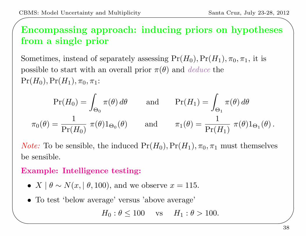
Encompassing approach: inducing priors on hypothesesfrom a single prior

Sometimes, instead of separately assessing Pr(H0),Pr(H1), π0, π1, it is

possible to start with an overall prior π(θ) and deduce the

Pr(H0),Pr(H1), π0, π1:

Pr(H0) =

∫Θ0

π(θ) dθ and Pr(H1) =

∫Θ1

π(θ) dθ

π0(θ) =1

Pr(H0)π(θ)1Θ0(θ) and π1(θ) =

1

Pr(H1)π(θ)1Θ1(θ) .

Note: To be sensible, the induced Pr(H0),Pr(H1), π0, π1 must themselves

be sensible.

Example: Intelligence testing:

• X | θ ∼ N(x, | θ, 100), and we observe x = 115.

• To test ‘below average’ versus ’above average’

H0 : θ ≤ 100 vs H1 : θ > 100.

38


&

$

%

• It is ‘known’ that θ ∼ N(θ | 100, 225).

• induced prior probabilities of hypotheses

Pr(H0) = Pr(θ ≤ 100) = 12 = Pr(H1)

• induced densities under each hypothesis:

π0(θ) = 2N(θ | 100, 225)I(−∞,100)(θ)

π1(θ) = 2N(θ | 100, 225)I(100,∞)(θ)

• Of course, we would not have needed to formally derive these.

– From the original encompassing prior π(θ), we can derive the

posterior and θ | x = 115 ∼ N(110.39, 69.23).

– Then directly compute the posterior probabilities:

Pr(H0 | x = 115) = Pr(θ ≤ 100 | x = 115) = 0.106

Pr(H1 | x = 115) = Pr(θ > 100 | x = 115) = 0.894

39


&

$

%

V. Paradoxes

40


&

$

%

Normal Example:

• Xi | θi.i.d.∼ N(xi | θ, σ2), σ2 known.

• Test H0 : θ = θ0 versus H1 : θ = θ0.

• Can reduce to sufficient statistic x ∼ N(x | θ σ2/n).

• Prior on H1: π1(θ) = N(θ | θ0, v20)

• Marginal likelihood under H1: m1(x) = N(x | θ0, v20 + σ2/n).

• posterior probability:

Pr(H0 | x) =

1 + Pr(H1)

Pr(H0)

1

(2π(v20+σ2/n))1/2

exp{− 1

21

v20+σ2/n

(x− θ0)2}

1

(2πσ2/n)1/2exp

{− 1

21

σ2/n(x− θ0)2

}−1

=

1 + Pr(H1)

Pr(H0)

exp{ 12z2 [1 + σ2

nv20]−1}

{1 + nv20/σ2}1/2

−1

,

where z =|x− θ0|σ/

√n

is the usual (frequentist) test statistic for this problem.

41


&

$

%

Comparing Pr(H0 | x) with classical p-value for various “n”

z p-value n = 5 n = 20 n = 100 Pr(H0 | x)

1.645 0.1 0.44 0.56 0.72 0.4121

1.960 0.05 0.33 0.42 0.60 0.32213

2.576 0.01 0.13 0.16 0.27 0.1334

where Pr(H0 | x) is the smallest Pr(H0 | x) can be among all normal priors

with mean θ0.

42


&

$

%

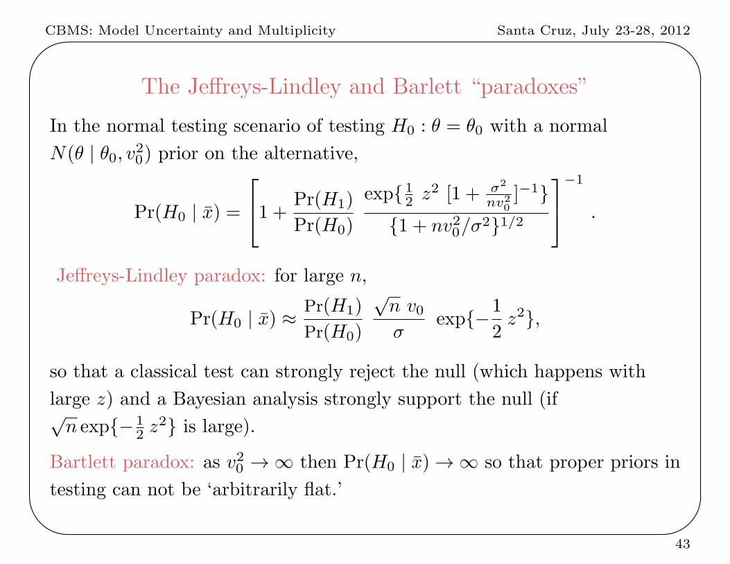
The Jeffreys-Lindley and Barlett “paradoxes”

In the normal testing scenario of testing H0 : θ = θ0 with a normal

N(θ | θ0, v20) prior on the alternative,

Pr(H0 | x) =

1 + Pr(H1)

Pr(H0)

exp{ 12 z2 [1 + σ2

nv20]−1}

{1 + nv20/σ2}1/2

−1

.

Jeffreys-Lindley paradox: for large n,

Pr(H0 | x) ≈ Pr(H1)

Pr(H0)

√n v0σ

exp{−1

2z2},

so that a classical test can strongly reject the null (which happens with

large z) and a Bayesian analysis strongly support the null (if√n exp{− 1

2 z2} is large).

Bartlett paradox: as v20 → ∞ then Pr(H0 | x) → ∞ so that proper priors in

testing can not be ‘arbitrarily flat.’

43


&

$

%

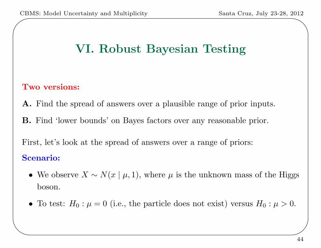
VI. Robust Bayesian Testing

Two versions:

A. Find the spread of answers over a plausible range of prior inputs.

B. Find ‘lower bounds’ on Bayes factors over any reasonable prior.

First, let’s look at the spread of answers over a range of priors:

Scenario:

• We observe X ∼ N(x | µ, 1), where µ is the unknown mass of the Higgs

boson.

• To test: H0 : µ = 0 (i.e., the particle does not exist) versus H0 : µ > 0.

44


&

$

%

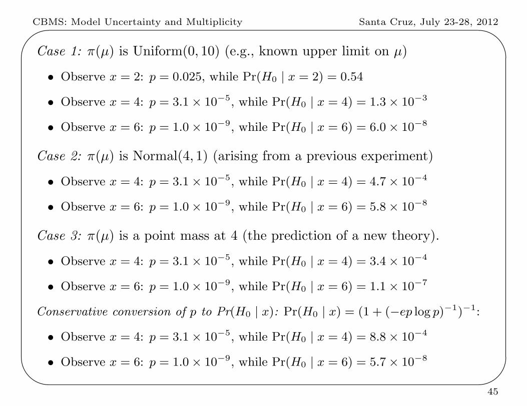
Case 1: π(µ) is Uniform(0, 10) (e.g., known upper limit on µ)

• Observe x = 2: p = 0.025, while Pr(H0 | x = 2) = 0.54

• Observe x = 4: p = 3.1× 10−5, while Pr(H0 | x = 4) = 1.3× 10−3


Case 2: π(µ) is Normal(4, 1) (arising from a previous experiment)



Case 3: π(µ) is a point mass at 4 (the prediction of a new theory).



Conservative conversion of p to Pr(H0 | x): Pr(H0 | x) = (1 + (−ep log p)−1)−1:



45


&

$

%

Lower bounds for the Normal Example:

• Xi | θi.i.d.∼ N(xi | θ, σ2), σ2 known.

• Test H0 : θ = θ0 versus H1 : θ = θ0.

• Prior on H1: π1(θ) = N(θ | θ0, v20)

– Mean of θ0 is natural (centering on the null), but choice of v20 is arbitrary.

• Bayes factor:

B01 =

√1 +

nv20σ2

exp{−1

2z2 [1 +

σ2

nv20]−1} .

where z =|x− θ0|σ/

√n

is the usual (frequentist) test statistic for this problem.

• Compute the minimum of B01 and Pr(H0 | x) over v20 :

For z > 1, the minimizing v20 is σ2

n (z2 − 1) (calculus) and

B 01 =√e z exp{− 1

2 z2} , Pr(H0 | x) = [1 +B−1

01 ]−1.

46


&

$

%

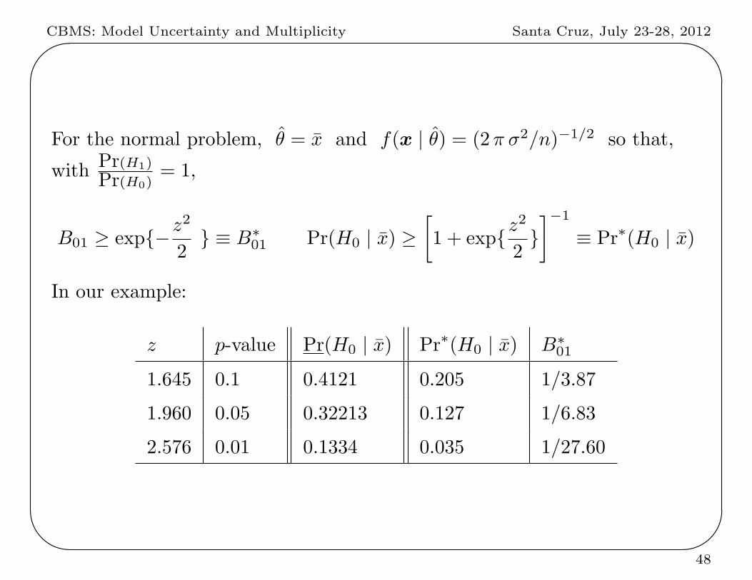
For the normal problem, θ = x and f(x | θ) = (2π σ2/n)−1/2 so that,

with Pr(H1)

Pr(H0)= 1,

B01 ≥ exp{−z2

2} ≡ B∗

01 Pr(H0 | x) ≥[1 + exp{z

2

2}]−1

≡ Pr∗(H0 | x)

In our example:

z p-value Pr(H0 | x) Pr∗(H0 | x) B∗01

1.645 0.1 0.4121 0.205 1/3.87

1.960 0.05 0.32213 0.127 1/6.83

2.576 0.01 0.1334 0.035 1/27.60

48


&

$

%

VII. Multiple Hypotheses and SequentialTesting

Two nice features of Bayesian testing:

• Multiple hypotheses can be easily handled.

• In sequential scenarios, there is no need to ‘spend α’ for looks at the

data; posterior probabilities are not affected by the reason for stopping

experimentation.

49


&

$

%

Normal testing example

The Xi are i.i.d from the N(xi | θ, 1) density, whereθ = mean effect of T1 - mean effect of T2

Standard Testing Formulation:

H0 : θ = 0 (no difference in treatments)

Ha : θ = 0 (a difference exists)

A More Revealing Formulation:

H0 : θ = 0 (no difference)

H1 : θ < 0 ( Treatment 2 is better)

H2 : θ > 0 ( Treatment 1 is better)

50


&

$

%

A default Bayesian analysis:

Prior Distribution:

• Assign H0 and Ha prior probabilities of 1/2 each

• On Ha, assign θ the “default” Normal(0,2) distribution (so that

Pr(H1) = Pr(H2) = 1/4)

Posterior Distribution:

After observing x = (x1, x2, . . . , xn), compute the posterior probabilities of

the various hypotheses, i.e.

Pr(H0 | x), Pr(H1 | x), Pr(H2 | x),

and Pr(Ha | x) = Pr(H0 | x) + Pr(H0 | x)

51


&

$

%

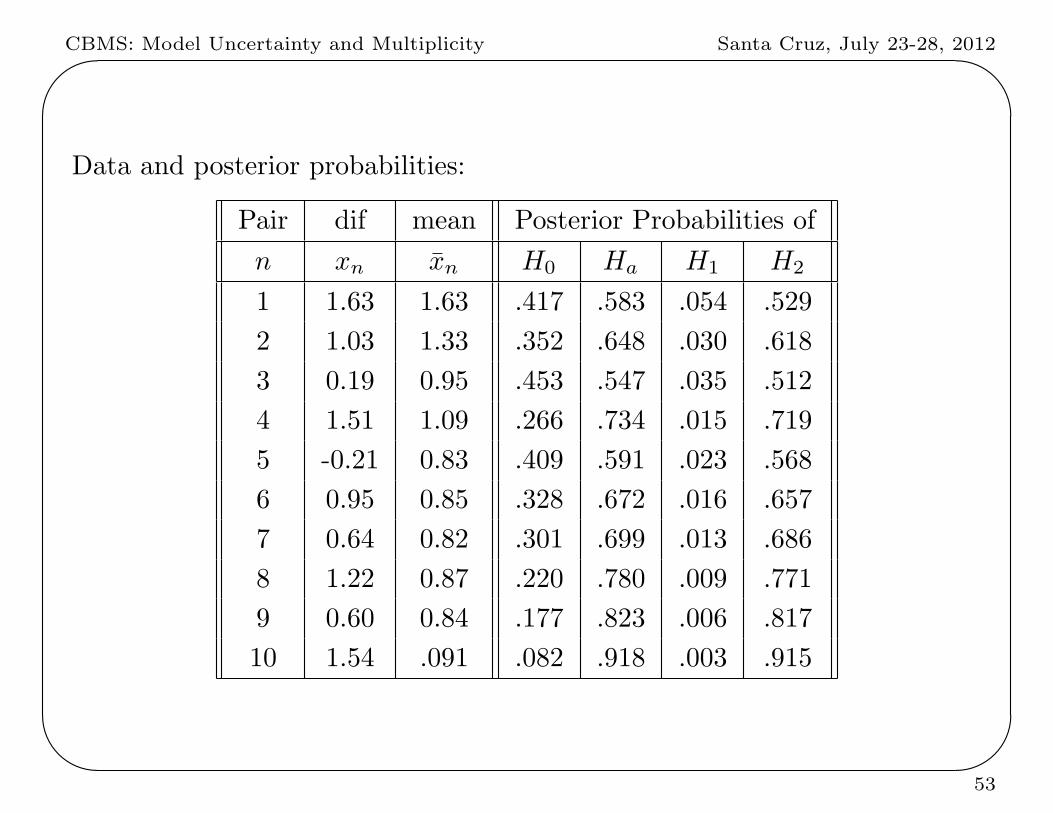
Data and posterior probabilities:

Pair dif mean Posterior Probabilities of

n xn xn H0 Ha H1 H2

1 1.63 1.63 .417 .583 .054 .529

2 1.03 1.33 .352 .648 .030 .618

3 0.19 0.95 .453 .547 .035 .512

4 1.51 1.09 .266 .734 .015 .719

5 -0.21 0.83 .409 .591 .023 .568

6 0.95 0.85 .328 .672 .016 .657

7 0.64 0.82 .301 .699 .013 .686

8 1.22 0.87 .220 .780 .009 .771

9 0.60 0.84 .177 .823 .006 .817

10 1.54 .091 .082 .918 .003 .915

53


&

$

%

Comments:

(i) Neither multiple hypothesis nor the sequential aspect caused

difficulties. There is no penalty (e.g. ‘spending α’) for looks at the data

(ii) Quantification of the support for H0 : θ = 0 is direct. At the 3rd

observations, Pr(H0 | x) = .453, at the end, Pr(H0 | x) = .082

(iii) H1 can be ruled out almost immediately

(iv) For testing H0 : θ = 0 versus Ha : θ = 0, the posterior probabilities are

frequentist error probabilities

54


&

$

%

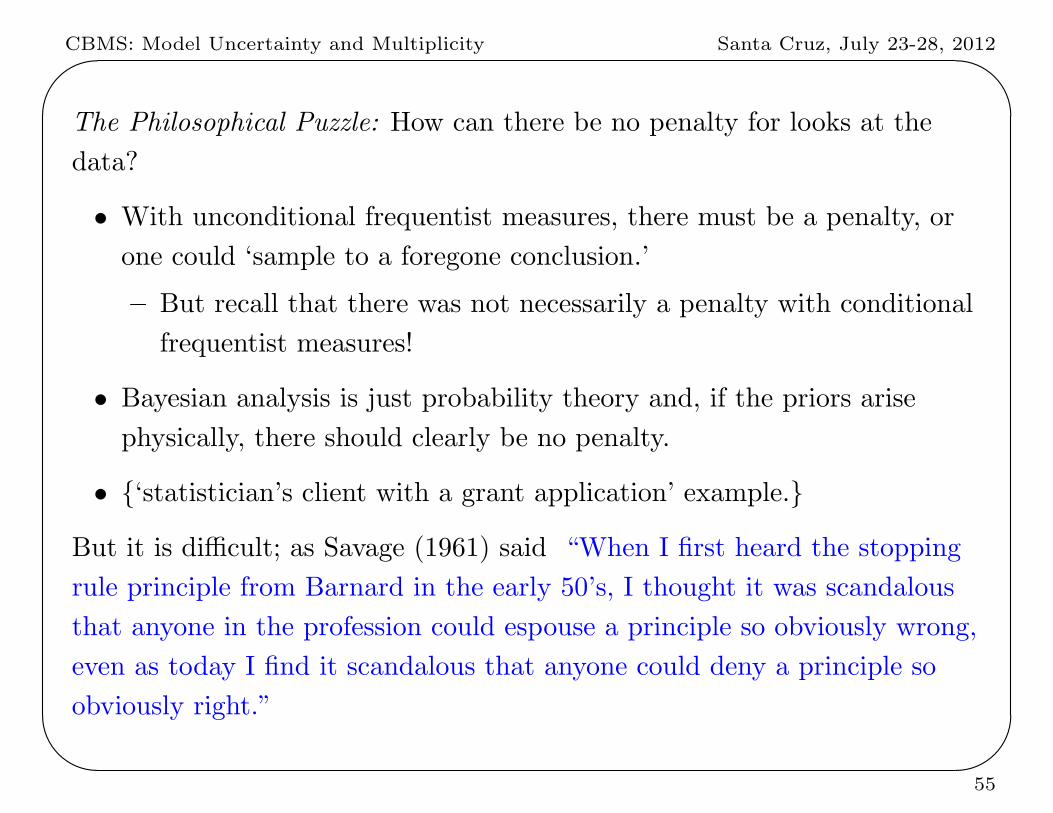
The Philosophical Puzzle: How can there be no penalty for looks at the

data?

• With unconditional frequentist measures, there must be a penalty, or

one could ‘sample to a foregone conclusion.’

– But recall that there was not necessarily a penalty with conditional

frequentist measures!

• Bayesian analysis is just probability theory and, if the priors arise

physically, there should clearly be no penalty.

• {‘statistician’s client with a grant application’ example.}

But it is difficult; as Savage (1961) said “When I first heard the stopping

rule principle from Barnard in the early 50’s, I thought it was scandalous

that anyone in the profession could espouse a principle so obviously wrong,

even as today I find it scandalous that anyone could deny a principle so

obviously right.”

55


&

$

%

VIII. HIV Vaccine Example

56


&

$

%57


&

$

%

Hypotheses, Data, and Classical Test:

• Alvac had shown no effect

• Aidsvax had shown no effect

Question: Would Alvac as a primer and Aidsvax as a booster work?

The Study: Conducted in Thailand with 16,395 individuals from the

general (not high-risk) population:

• 74 HIV cases reported in the 8198 individuals receiving placebos

• 51 HIV cases reported in the 8197 individuals receiving the treatment

Model: X1 ∼ Binomial(x1 | p1, 8198) and X2 ∼ Binomial(x2 | p2, 8197),respectively, so that p1 and p2 denote the probability of HIV in the placebo

and treatment populations, respectively.

Classical test of H0 : p1 = p2 versus H1 : p1 = p2 yielded a p-value of 0.04.

58


&

$

%

Bayesian Analysis: Reparameterize to p1 and V = 100(1− p2

p1

),

so that we are testing

H0 : V = 0, p1 arbitrary

H1 : V = 0, p1 arbitrary.

Prior distribution:

• Pr(Hi) = prior probability that Hi is true, i = 0, 1,

• Let π0(p1) = π1(p1), and choose them to be either

– uniform on (0,1)

– subjective (evidence-based?) priors based on knowledge of HIV

infection rates

Note: the answers are essentially the same for either choice.

• For V under H1, consider the priors

– uniform on (-20, 60) (apriori subjective – evidence-based – beliefs)

– uniform on (−100c/3, 100c) for 0 < c < 1, to study sensitivity

(constrained also to V > 100(1− 1p1).

59


&

$

%

Posterior probability of the null hypothesis:

Pr(H0 | data) = Pr(H0)B01

Pr(H0)B01 + Pr(H1),

where the Bayes factor of H0 to H1 is

B01 =

∫Binomial(74 | p1, 8198)Binomial(51 | p1, 8197)π0(p1)dp1∫

Binomial(74 | p1, 8198)Binomial(51 | p2, 8197)π0(p1)π1(p2 | p1)dp1dp2.

• For the prior for V that is uniform on (-20, 60),

B01 ≈ 1/4 ( recall, p-value ≈ .04)

• If the prior probabilitites of the hypotheses are each 1/2, the overall

posterior density of V has

– a point mass of size 0.20 at V = 0,

– a density (having total mass 0.80) on non-zero values of V :

60


&

$

%−20 0 20 40 60

0.0

1.0

2.0

VE

prob

abilit

y den

sity o

f VE

RV144 data; no adjustment

0.2

61


&

$

%

Robust Bayes: For the prior on V that is uniform on (−100c/3, 100c),

the Bayes factor is

0.0 0.2 0.4 0.6 0.8 1.0

0.2

0.6

1.0

c

B_0

1(c)

Thai B01; psi ~ Un(−c/3, c)

Note: There is sensitivity to c, indeed 0.22 < B01(c) < 1, but why would

this cause one to instead report p = 0.04, knowing it will be misinterpreted?

Note: Uniform priors are the extreme points of monotonic priors, and so

such robustness curves are quite general.

62


&

$

%

Alternative frequentist perspective:

Let α and (1− β(θ)) be the Type I error and power for testing H0 versus

H1 with, say, rejection region R = {z : z > 1.645}. Then

O = Odds of correct rejection to incorrect rejection

= [prior odds of H1 to H0]×(1− β)

α,

where (1− β) =∫(1− β(θ))π(θ)dθ is average power wrt the prior π(θ).

• (1−β)α =

average powertype 1 error is the experimental odds of correct rejection to

incorrect rejection.

• For vaccine example, (1− β) = 0.45 and α = 0.05 (the error probability

corresponding to R), so (1−β)α = 9.

average power 0.05 0.25 0.50 0.75 1.0 0.01 0.25 0.50 0.75 1.0

type I error 0.05 0.05 0.05 0.05 0.05 0.01 0.01 0.01 0.01 0.01

correct/incorrect 1 5 10 15 20 1 25 50 75 100

63


&

$

%

But that is pre-experimental; better is to report the actual data-based odds

of correct rejection to incorrect rejection, namely the Bayes factor B10(z).

• For vaccine example, here is B10(z) (recall(1−β)

α = 9):

1.6 1.8 2.0 2.2 2.4 2.6 2.8 3.0

510

1520

2530

35

x

BF

(x)

• For simple nulls (or nulls that are simple for the test statistic)

E[B10(Z) | H0,R] = (1−β)α , so reporting B10(z) is a valid conditional

frequentist procedure. (Kiefer, 1977 JASA; Brown, 1978 AOS)

64


&

$

%

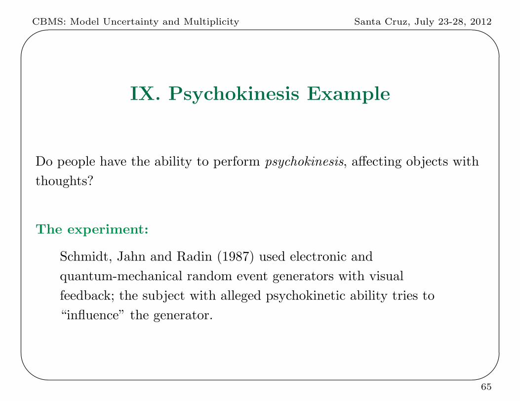
IX. Psychokinesis Example

Do people have the ability to perform psychokinesis, affecting objects with

thoughts?

The experiment:

Schmidt, Jahn and Radin (1987) used electronic and

quantum-mechanical random event generators with visual

feedback; the subject with alleged psychokinetic ability tries to

“influence” the generator.

65


&

$

%

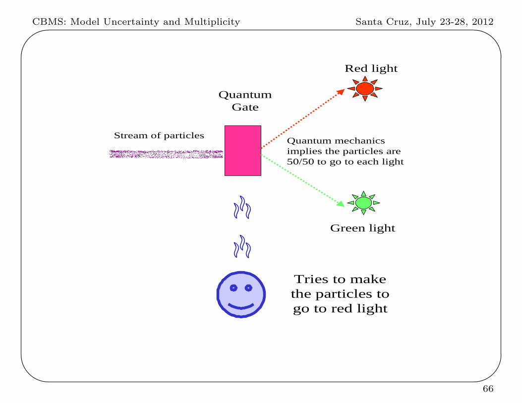
Stream of particles

QuantumGate

Red light

Green light

Quantum mechanicsimplies the particles are50/50 to go to each light

Tries to makethe particles togo to red light

Á Á

66


&

$

%

Data and model:

• Each “particle” is a Bernoulli trial (red = 1, green = 0)

θ = probability of “1”

n = 104, 490, 000 trials

X = # “successes” (# of 1’s), X ∼ Binomial(n, θ)

x = 52, 263, 470 is the actual observation

To test H0 : θ = 12 (subject has no influence)

versus H1 : θ = 12 (subject has influence)

• P-value = Pθ= 12(|X − n

2 | ≥ |x− n2 |) ≈ .0003.

Is there strong evidence against H0 (i.e., strong evidence that the

subject influences the particles) ?

67


&

$

%

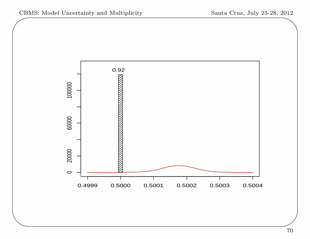
Bayesian Analysis: (Jefferys, 1990)

Prior distribution:

Pr(Hi) = prior probability that Hi is true, i = 0, 1;

On H1 : θ = 12 , let π(θ) be the prior density for θ.

Subjective Bayes: choose the Pr(Hi) and π(θ) based on personal beliefs

Objective (or default) Bayes: choose

Pr(H0) = Pr(H1) =12

π(θ) = 1 (on 0 < θ < 1)

68


&

$

%0.4999 0.5000 0.5001 0.5002 0.5003 0.5004

020

000

6000

010

0000

0.92

70


&

$

%

Bayes Factor:

B01 = likelihood of observed data under H0

‘average′ likelihood of observed data under H1

=f(x | θ= 1

2)∫ 1

0 f(x | θ)π(θ)dθ≈ 12

Crash of frequentist and Bayesian conclussions is dramatic.

• α0 ≤ 0.5 requires π1 ≥ 0.92,

• alternatively ; require a π(θ) under H1 extremely concentrated around

H0 : θ = 0.5 (that is, both hypothesis would then be very precise)

71


&

$

%

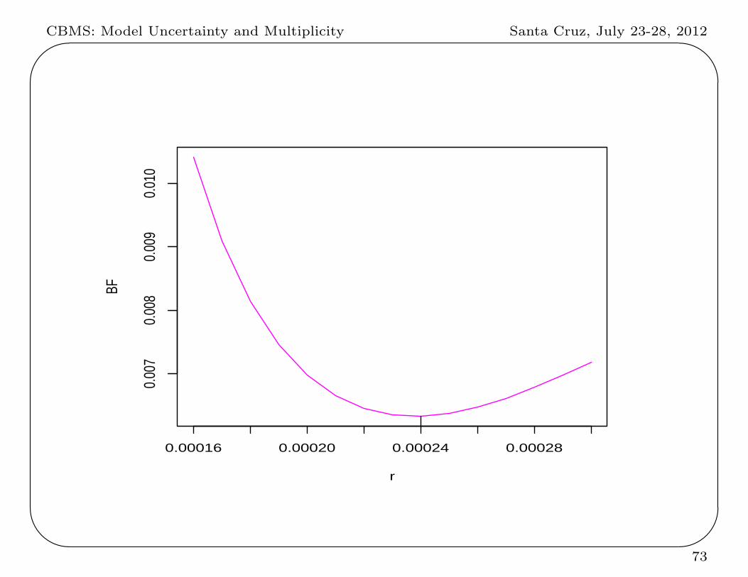
Choice of the prior density or weight function, π, on {θ : θ = 1

2}

Consider πr(θ) = U(θ | 12 − r, 1

2 + r) the uniform density on (12 − r, 12 + r)

Subjective interpretation: r is the largest chance in success probability

that you would expect, given that ESP exists. And you give equal

probability to all θ in the interval (12 − r, 12 + r) .

Resulting Bayes factor (letting FBe(· | a, b) denote the CDF of the

Beta(a, b) distribution)

B(r) =f(x | 1/2)∫ 1

0f(x | θ)πr(θ) dθ

=

(n

x

)(n+ 1) r

2n−1[FB2 − FB1]

−1

where

FB2 = FBe( 12 + r | x+ 1, n− x+ 1) and

FB1 = FBe( 12 − r | x+ 1, n− x+ 1)

For example, B(0.25) ≈ 6

72


&

$

%0.00016 0.00020 0.00024 0.00028

0.00

70.

008

0.00

90.

010

r

BF

73


&

$

%

r = largest increase in success probability that would be expected, given

ESP exists.

the minimum value of B(r) is 1158 , attained at the minimizing value of

r = .00024

Conclusion: Although the p-value is small (.0003), for typical prior beliefs

the data would provide evidence for the simpler model H0 : no ESP.

Only if one believed a priori that |θ − 12 | ≤ .0021, would the evidence

for H1 be at least 20 to 1.

74


&

$

%

X. More on p-values and their Calibration

75


&

$

%

Background concerns with p-values

• Concerns with use of p-values trace back to at least Berkson (1937).

• Concerns are recurring in many scientific literatures:

Environmental sciences: http://www.indiana.edu/∼stigtsts/

Social sciences: http://acs.tamu.edu/∼bbt6147/

Wildlife science: http://www.npwrc.usgs.gov/perm/hypotest/

http://www.cnr.colostate.edu/∼anderson/null.html

• Numerous works specifically focus on comparing the Fisher and N-P

approaches (e.g., Lehmann, 1993 JASA: The Fisher, N-P Theories of Testing

Hypotheses: One Theory or Two?)

• Even the popular press has become involved: The Sunday Telegraph,

September 13, 1998:

76


&

$

%77


&

$

%

Commonly aired issues with p-values

• Inappropriate fixation with p = 0.05.

• p-values do not measure the magnitude or importance of the effect

being investigated.

• p-values are commonly misinterpreted as

– the probability that H0 is true, given the data;

– the probability an error is made in rejecting H0;

– the probability that a ‘replicating’ experiment would reach the same

conclusion.

Cohen (1994): The statistical significance test “does not tell us what we

want to know, and we so much want to know what we want to know that,

out of desperation, we nevertheless believe that it does!”

78


&

$

%

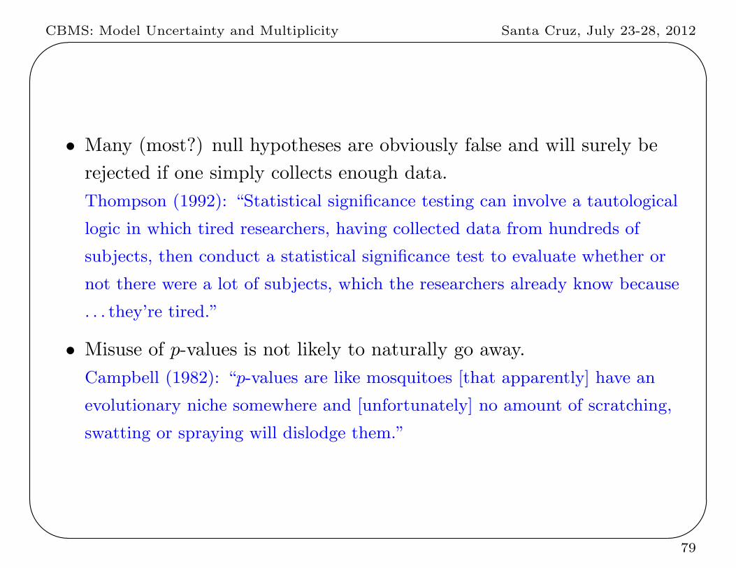
• Many (most?) null hypotheses are obviously false and will surely be

rejected if one simply collects enough data.

Thompson (1992): “Statistical significance testing can involve a tautological

logic in which tired researchers, having collected data from hundreds of

subjects, then conduct a statistical significance test to evaluate whether or

not there were a lot of subjects, which the researchers already know because

. . . they’re tired.”

• Misuse of p-values is not likely to naturally go away.

Campbell (1982): “p-values are like mosquitoes [that apparently] have an

evolutionary niche somewhere and [unfortunately] no amount of scratching,

swatting or spraying will dislodge them.”

79


&

$

%

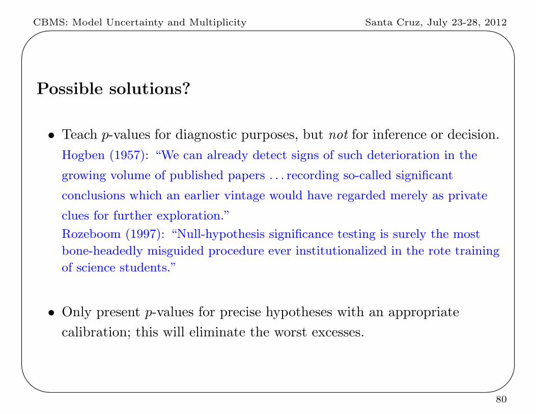
Possible solutions?

• Teach p-values for diagnostic purposes, but not for inference or decision.

Hogben (1957): “We can already detect signs of such deterioration in the

growing volume of published papers . . . recording so-called significant

conclusions which an earlier vintage would have regarded merely as private

clues for further exploration.”

Rozeboom (1997): “Null-hypothesis significance testing is surely the most

bone-headedly misguided procedure ever institutionalized in the rote training

of science students.”

• Only present p-values for precise hypotheses with an appropriate

calibration; this will eliminate the worst excesses.

80


&

$

%

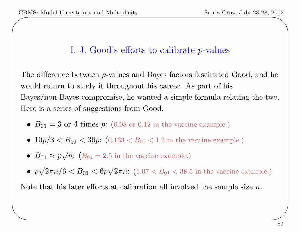
I. J. Good’s efforts to calibrate p-values

The difference between p-values and Bayes factors fascinated Good, and he

would return to study it throughout his career. As part of his

Bayes/non-Bayes compromise, he wanted a simple formula relating the two.

Here is a series of suggestions from Good.

• B01 = 3 or 4 times p: (0.08 or 0.12 in the vaccine example.)

• 10p/3 < B01 < 30p: (0.133 < B01 < 1.2 in the vaccine example.)

• B01 ≈ p√n: (B01 = 2.5 in the vaccine example.)

• p√2πn/6 < B01 < 6p

√2πn: (1.07 < B01 < 38.5 in the vaccine example.)

Note that his later efforts at calibration all involved the sample size n.

81


&

$

%

Calibration of p-values from Vovk (1993 JRSSB) and Sellke,Bayarri and Berger (2001 Am. Stat.)

• A proper p-value satisfies H0 : p(X) ∼ Uniform(0, 1).

• Test versus H1 : p(X) ∼ Beta(ξ, 1), 0 < ξ < 1. Then, when p < e−1,

B01(p) =1

ξp(ξ−1)≥ −e p log(p) .

This bound also holds for any alternative f(p), where Y = − log(p) has

a decreasing failure rate (natural non-parametric alternatives).

• The corresponding bound on the conditional Type I frequentist error is

α ≥ (1 + [−e p log(p)]−1)−1 .

p .2 .1 .05 .01 .005 .001 .0001 .00001

−ep log(p) .879 .629 .409 .123 .072 .0189 .0025 .00031

α(p) .465 .385 .289 .111 .067 .0184 .0025 .00031

82


&

$

%Figure 2: J.P. Ioannides: Am J Epidemiol 2008;168:374–383

83


&

$

%84


&

$

%85


&

$

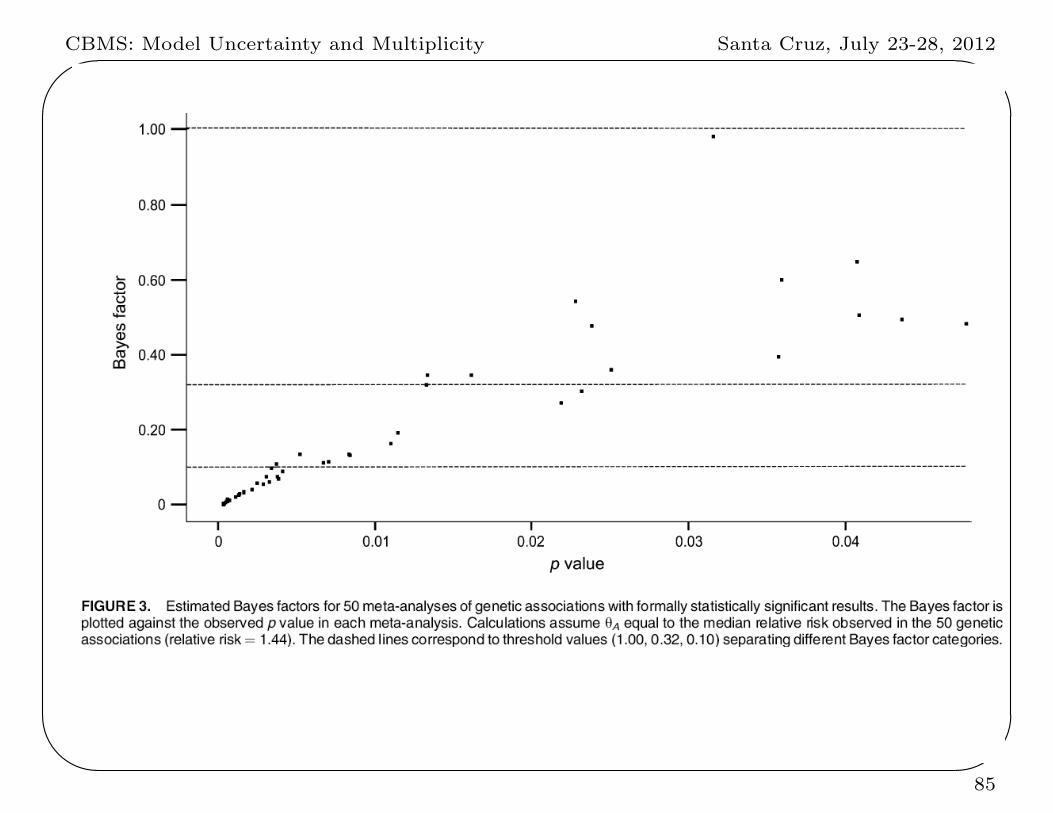
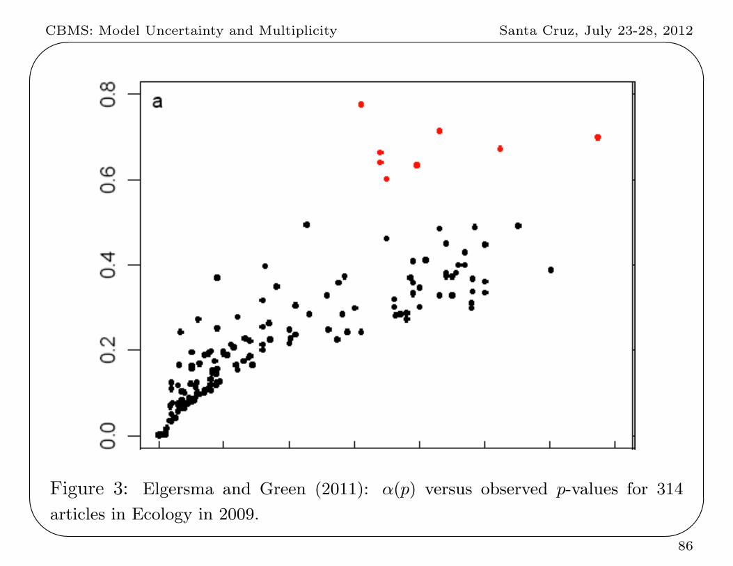
%Figure 3: Elgersma and Green (2011): α(p) versus observed p-values for 314

articles in Ecology in 2009.

86


&

$

%

Two legitimate uses of p-values

• As an indication that something unusual has happened and one should

investigate further.

– Very useful at initial stages of the analysis:

∗ If p is not small, don’t proceed.

∗ If it is small, perform the Bayesian analysis. (I would argue

always; physics a year ago had an 8σ result that didn’t replicate.)

– It would be better to measure ‘unusual’ by −ep log p.

• As a statistic to measure ‘strength of evidence’, for use in conditional

frequentist testing; indeed, it yields conditional frequentist tests that

are exactly the same as objective Bayesian tests. (This was the story

about how use of Fisher’s p-value and conditioning ideas, when

combined with Neyman’s frequentist testing formulation, results in

identical answers as Jeffreys objective Bayesian testing.)

87

Lecture 2: Bayesian Hypothesis Testing - CBMS-MUM · ’CBMS: Model Uncertainty and Multiplicity...

Documents

Transcript of Lecture 2: Bayesian Hypothesis Testing - CBMS-MUM · ’CBMS: Model Uncertainty and Multiplicity...