Lecture 19Search Theoretic Models of Money

Noah Williams

University of Wisconsin - Madison

Economics 712

Williams Economics 712

.

Essential Models of Money

• Hahn (1965): money is essential if it allows agents to achieve allo-cations they cannot achieve with other mechanisms that also respectthe enforcement and information constraints in the environment.

• Why do we care about essential models of money?

• Three frictions that will make money essential:

1. Double-coincidence of wants problem.

2. Long-run commitment cannot be enforced.

3. Agents are anonymous: histories are not public information.

• Money is a consequence of these frictions in trade: medium of ex-change.

3

Three Generations of Models

1. 1 unit of money, 1 unit of good: Kiyotaki and Wright (1993).

2. 1 unit of money, endogenous units of good: Trejos and Wright (1995).

3. Endogenous units of money, endogenous units of good: Lagos and

Wright (2005).

4

Environment

• [0, 1] continuum of anonymous agents.

• Live forever and discount future at rate r.

• [0, 1] continuum of goods. Good i is produced by agent i.

• Goods are non-storable: no commodity money.

• Unit cost of production c ≥ 0.

5

.

Double-Coincidence of Wants Problem

• I do not produce what I like (non-restrictive: home production, spe-cialization).

• iWj: agent i likes to consume good produced by agent j :.

1. utility u > c from consuming j.

2. utility 0 otherwise.

• Probabilities of matching:

p (iWi) = 0

p (jWi) = x

p (jWi|iWj) = y

6

First Generation: Fixed Money and Fixed Good

• Exogenously given quantityM ∈ [0, 1] of an indivisible unit of storablegood.

• Holding money yields zero utility γ: fiat money.

• Initial endowment: M agents are randomly endowed with one unit of

money.

• Agents holding money cannot produce (for example because you needto consume before you can produce again).

• We eliminate (non-trivial) distributions.

7

Trades

• Pairwise random matching of agents with Poisson arrival time α.

• Bilateral trading is important, randomness is not (Corbae, Temzelides,Wright, 2003).

• Upon meeting, agents decide whether to trade. Then, they part com-pany and re-enter the process.

• History of previous trades is unknown.

• Exchange 1 unit of good for 1 unit of good (barter) or 1 unit of money.8

Individual Trading Strategies

• Agents never accept a good in trade if he does not like to consume itsince it is not storable.

• They will barter if they like the both agents in the pair like each othergoods.

• Would they accept money for goods and viceversa?

• We will look at stationary and symmetric Nash equilibria.

9

Probabilities

• You meet someone with arrival rate α.

• This person can produce with probability 1−M.

• With probability x you like what he produces.

• With probability π = π0π1 (endogenous objects to be determined)

both of you want to trade.

• If π > 0, we say that money circulates.10

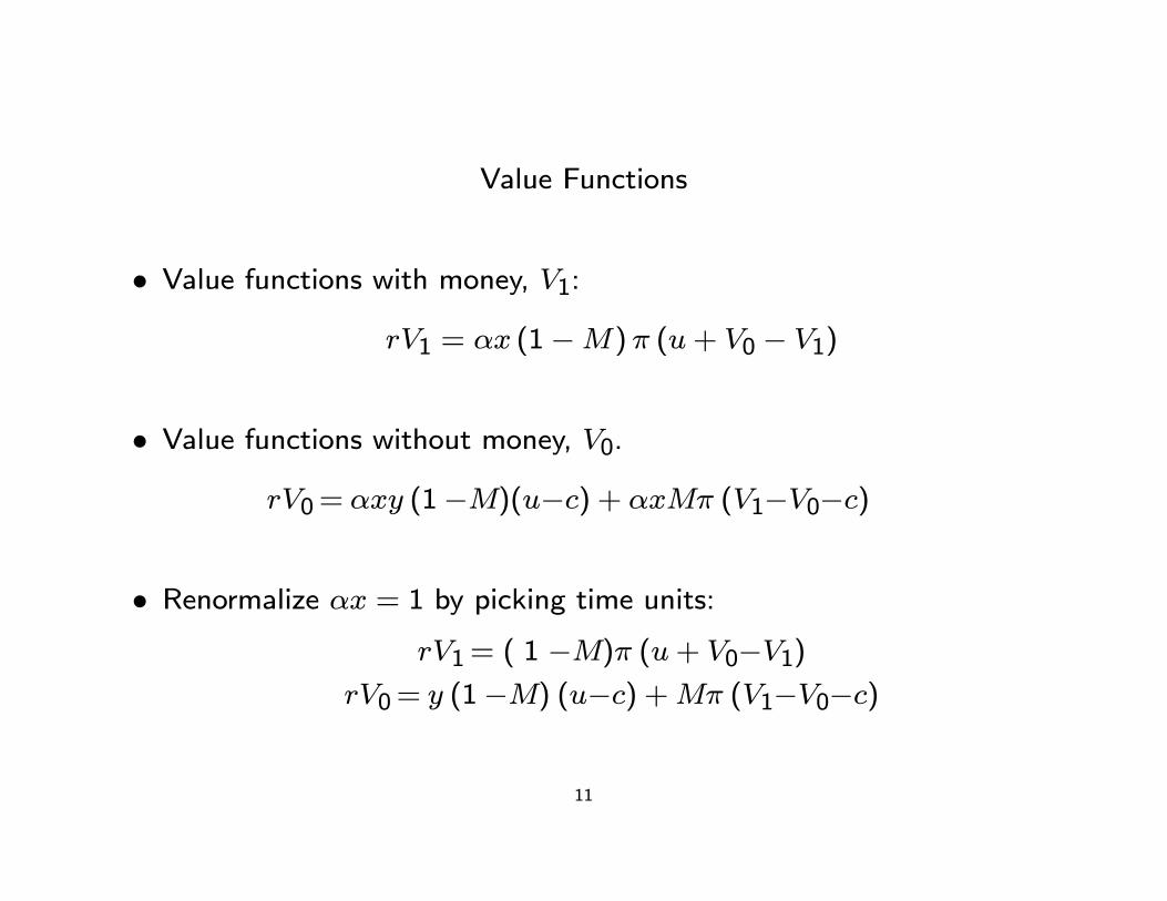
Value Functions

• Value functions with money, V1:

rV1 = αx (1−M)π (u+ V0 − V1)

• Value functions without money, V0.

rV0 = αxy (1 −M)(u−c) + αxMπ (V1−V0−c)

• Renormalize αx = 1 by picking time units:rV1 = ( 1 −M)π (u + V0−V1)

rV0 = y (1 −M) (u−c) +Mπ (V1−V0−c)

11

Individual Trading Strategies

• Net gain from trading goods for money:

∆0 = V1 − V0 − c =(1−M) (π − y) (u− c)− rc

r + π

• Net gain from trading money from goods:

∆1 = u+ V0 − V1 =(Mπ + (1−M) y) (u− c) + ru

r + π

12

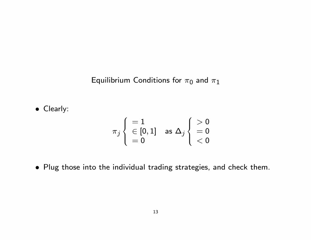
Equilibrium Conditions for π0 and π1

• Clearly:

πj

⎧⎪⎨⎪⎩= 1∈ [0, 1]= 0

as ∆j

⎧⎪⎨⎪⎩> 0= 0< 0

• Plug those into the individual trading strategies, and check them.

13

Characterizing π

• Clearly ∆1 > 0. Hence π1 = 1, i.e., the agent with money always

wants to trade.

• For π0, you have

∆0 =(1−M) (u− c)π0

r + π0− (1−M) y (u− c) + rc

r + π0

• Then, ∆0 has the same sign as

π0 −rc+ (1−M) y (u− c)(1−M) (u− c)

= π0 − bπ14

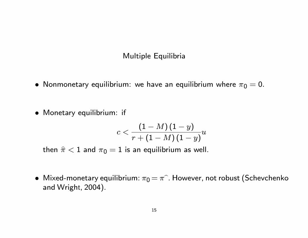
Multiple Equilibria

• Nonmonetary equilibrium: we have an equilibrium where π0 = 0.

• Monetary equilibrium: if

c <(1−M) (1− y)

r + (1−M) (1− y)u

then bπ < 1 and π0 = 1 is an equilibrium as well.

• Mixed-monetary equilibrium: π0 = πb. However, not robust (Schevchenko and Wright, 2004).

15

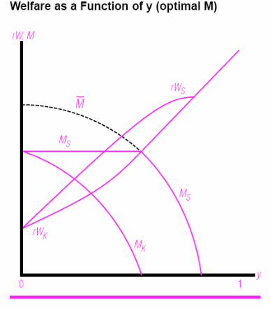
Welfare

• Define welfare as the average utility:

W =MV1 + (1−M)V0

• Then:

rW = (1−M) [(1−M) y +Mπ] (u− c)

• Note that welfare is increasing in π.

16

Welfare π = 1

• Note:rW = ( 1 −M) [ ( 1

2

−M)y + M] (u−c)

• Maximize W with respect to M :

M∗ =1− 2y2− 2y

if y <1

2

M∗ = 0 if y ≥ 1

2

• Intuition: facilitate trade versus crowding out barter.17

Welfare π = 0

• Note:

rW = (1−M) [(1−M) y] (u− c)

• Monotonically decreasing in M ⇒M∗ = 0.

• Result is a little bit silly: it depends on the absence of free disposal ofmoney. Otherwise, welfare is independent of M.

18

Welfare π

• Note:

rW = (1−M) [(1−M) y +Mπ] (u− c)

• Monotonically increasing in M in the [0, M] interval.

19

Define M such that π=1,

Comparison with Alternative Arrangements

• Imagine that we have the credit arrangement: “produce for anyoneyou meet that wants your good.”

• Value function

rVc = u− c

• Clearly

rVc > rW

• However, this arrangement is not self-enforceable: histories are notobserved.

20

Second Generation: Endogenous Prices

• We make the very strong assumption that we exchanged one good forone unit of money.

• What if we let prices be endogenous? Shi (1995) and Trejos and Wright (1995).

• We set y = 0 and we let goods be divisible.

• When agents meet, they bargain about how much q will be exchanged,or equivalently, about price 1/q.

21

Utility and Cost Functions

• Utility is u (q) and cost of production is c (q) .

• Assumptions:u (0) = c (0) = 0 u0 (0) > c ' (0)

u0 (0) > 0, u00 (0) ≤ 0c0 (0) > 0, c00 (0) ≥ 0

• Also, bq and q∗ are such thatu(qb) = c(qb) u0(q∗) = c0(q∗)

22

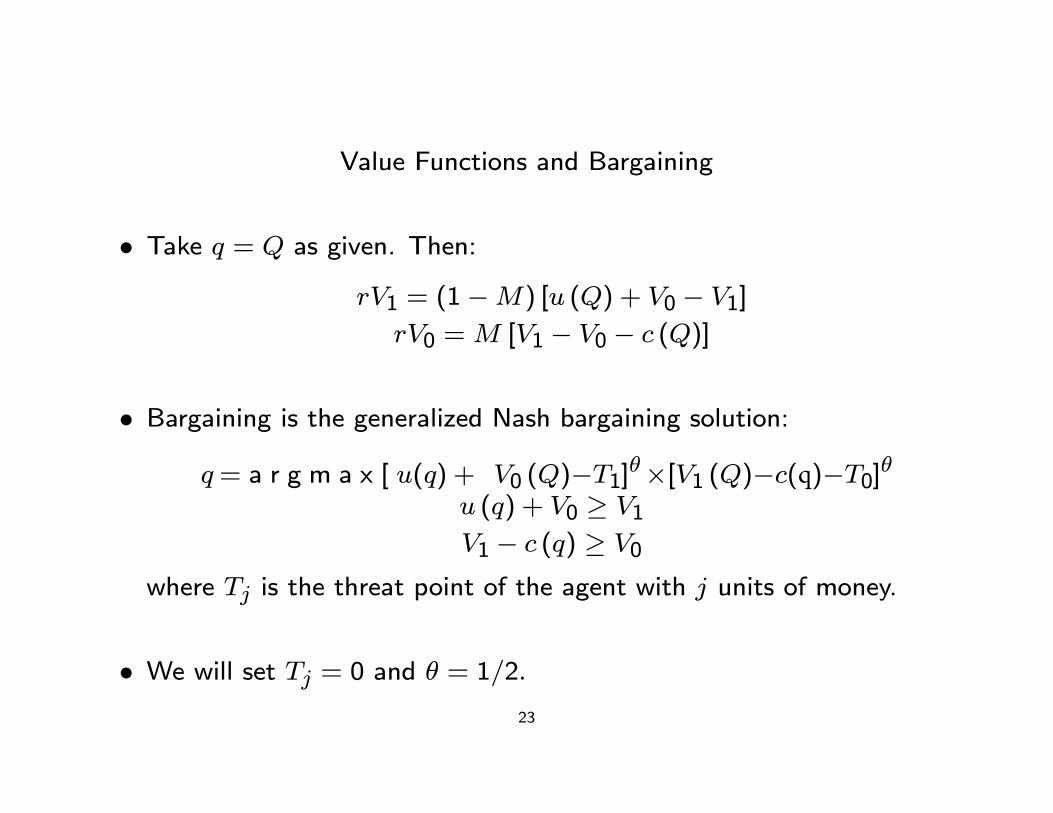
Value Functions and Bargaining

• Take q = Q as given. Then:

rV1 = (1−M) [u (Q) + V0 − V1]rV0 =M [V1 − V0 − c (Q)]

• Bargaining is the generalized Nash bargaining solution:

q = a r g m a x [ u(q) + V0 (Q)−T1]θ ×[V1 (Q)−c(q)−T0]θu (q) + V0 ≥ V1V1 − c (q) ≥ V0

where Tj is the threat point of the agent with j units of money.

• We will set Tj = 0 and θ = 1/2.

23

Equilibria

• Necessary condition taking V0 (Q) and V1 (Q) as given:

[V1 (Q)− c (q)]u0 (q) = [u (q) + V0 (Q)] c0 (q)

• The bargaining solution defines a function

q = e (Q)

and we look at its fixed points.

• Two fixed points:

1. q = 0: nonmonetary equilibrium.

2. q = qe > 0: monetary equilibrium.

24

Efficiency

• Note that the efficient outcome is q∗, i.e. u0 (q∗) = c0 (q∗) .

• In the monetary equilibrium:

u0 (qe) =u (qe) + V0 (q

e)

V1 (qe)− c (qe)c0 (qe) > u0 (q∗)

since u (qe) + V0 (qe) > V1 (q

e)− c (qe) .

• Hence q∗ > qe, or equivalenty, the price is too high.

25

Third Generation: Endogenous Prices and Goods

• Relax the assumption that agents hold 0 or 1 units of money.

• Problem: endogenous distribution of money that we (and the agents!)need to keep track of.

• Computational: Molico (2006).

• Theoretical:

1. Families: Shi (1997).

2. Two markets: Lagos and Wright (2005).

26