Lecture 19 -- Interfacing MATLAB with CAD
35
4/3/2018 1 ECE 5322 21 st Century Electromagnetics Instructor: Office: Phone: E‐Mail: Dr. Raymond C. Rumpf A‐337 (915) 747‐6958 [email protected] Synthesizing Geometries for 21st Century Electromagnetics Interfacing MATLAB with CAD Lecture #19 Lecture 19 1 Lecture Outline • STL Files – File format description – Problems and repairing • MATLAB Topics – Importing and exporting STL files in MATLAB – Visualizing surface meshes in MATLAB – Generating faces and vertices using MATLAB – Surface mesh 3D grid • CAD Topics – Converting flat images to STL – Point clouds – Importing custom polygons into SolidWorks – STL to CAD file conversion Lecture 19 Slide 2
-
Upload
nguyenkhue -
Category
Documents
-
view
232 -
download
0
Transcript of Lecture 19 -- Interfacing MATLAB with CAD

4/3/2018
1
ECE 5322 21st Century Electromagnetics
Instructor:Office:Phone:E‐Mail:
Dr. Raymond C. RumpfA‐337(915) 747‐[email protected]
Synthesizing Geometries for 21st Century Electromagnetics
Interfacing MATLAB with CAD
Lecture #19
Lecture 19 1
Lecture Outline• STL Files
– File format description– Problems and repairing
• MATLAB Topics– Importing and exporting STL files in MATLAB– Visualizing surface meshes in MATLAB– Generating faces and vertices using MATLAB– Surface mesh 3D grid
• CAD Topics– Converting flat images to STL– Point clouds– Importing custom polygons into SolidWorks– STL to CAD file conversion
Lecture 19 Slide 2

4/3/2018
2
STL File Format Description
What is an STL File?
Lecture 19 Slide 4
STL – Standard Tessellation Language
This file format is widely used in rapidprototyping (i.e. 3D printing, additive manufacturing). It contains only a single triangular mesh of an objects surface. Color, texture, materials, and other attributes are not represented in the standard STL file format. Hacked formats exists to accommodate this type of additional information.
They can be text files or binary. Binary is more common because they are more compact. We will look at text files because that is more easily interfaced with MATLAB.

4/3/2018
3
Surface Mesh
Lecture 19 5
Despite this sphere really being a solid object, it is represented in an STL file by just its surface.
Solid Object
STL Representation
STL File Format
Lecture 19 6
solid name
facet normal nx ny nzouter loop
vertex vx,1 vy,1 vz,1vertex vx,2 vy,2 vz,2vertex vx,3 vy,3 vz,3
endloopendfacet
endsolid name
This set of text is repeated for every triangle on the surface of the object.
1v
2v 3v
Bold face indicates a keyword; these must appear in lower case. Note that there is a space in “facet normal” and in “outer loop,” while there is no space in any of the keywords beginning with “end.” Indentation must be with spaces; tabs are not allowed. The notation, “{…}+,” means that the contents of the brace brackets can be repeated one or more times. Symbols in italics are variables which are to be replaced with user-specified values. The numerical data in the facet normal and vertex lines are single precision floats, for example, 1.23456E+789. A facet normal coordinate may have a leading minus sign; a vertex coordinate may not.
2 1 3 1
2 1 3 1
ˆv v v v
v v v vn

4/3/2018
4
Example STL File
Lecture 19 Slide 7
solid pyramidfacet normal -8.281842e-001 2.923717e-001 -4.781524e-001
outer loopvertex 4.323172e-018 1.632799e-017 6.495190e-001vertex 3.750000e-001 7.081604e-001 4.330127e-001vertex 3.750000e-001 0.000000e+000 0.000000e+000
endloopendfacetfacet normal 0.000000e+000 2.923717e-001 9.563048e-001
outer loopvertex 7.500000e-001 0.000000e+000 6.495190e-001vertex 3.750000e-001 7.081604e-001 4.330127e-001vertex 0.000000e+000 0.000000e+000 6.495190e-001
endloopendfacetfacet normal 8.281842e-001 2.923717e-001 -4.781524e-001
outer loopvertex 3.750000e-001 -1.632799e-017 0.000000e+000vertex 3.750000e-001 7.081604e-001 4.330127e-001vertex 7.500000e-001 0.000000e+000 6.495190e-001
endloopendfacetfacet normal 0.000000e+000 -1.000000e+000 0.000000e+000
outer loopvertex 3.750000e-001 0.000000e+000 0.000000e+000vertex 7.500000e-001 0.000000e+000 6.495190e-001vertex 0.000000e+000 0.000000e+000 6.495190e-001
endloopendfacet
endsolid pyramid
An STL file is essentially just a list of all the triangles on the surface of an object.
Each triangle is defined with a surface normal and the position of the three vertices.
A Single Triangle
Lecture 19 Slide 8
facet normal -8.281842e-001 2.923717e-001 -4.781524e-001outer loop
vertex 4.323172e-018 1.632799e-017 6.495190e-001vertex 3.750000e-001 7.081604e-001 4.330127e-001vertex 3.750000e-001 0.000000e+000 0.000000e+000
endloopendfacet
Vertex 1
Vertex 3
Vertex 2
Facet Normal1. Facet normal must follow right‐hand
rule and point outward from object.a) Some programs set this to [0;0;0]
or convey shading information.b) Don’t depend on it!
2. Adjacent triangles must have two common vertices.
3. STL files appear to be setup to handle arbitrary polygons. Don’t do this.

4/3/2018
5
Warnings About Facet Normals
• Since the facet normal can be calculated from the vertices using the right-hand rule, sometimes the facet normal in the STL file contains other information like shading, color, etc.
• Don’t depend on the right-hand rule being followed.
• Basically, don’t depend on anything!
Lecture 19 9
STL File Problems and
Repairing

4/3/2018
6
Inverted Normals
Lecture 19 11
All surface normals should point outwards.
Good Bad
http://admproductdesign.com/workshop/3d‐printing/definition‐of‐stl‐errors.html
Intersecting Triangles
Lecture 19 12
No faces should cut through each other. Intersections should be removed.
http://admproductdesign.com/workshop/3d‐printing/definition‐of‐stl‐errors.html

4/3/2018
7
Noise Shells
Lecture 19 13
A shell is a collection of triangles that form a single independent object. Some STL files may contain small shells that are just noise. These should be eliminated.
Main shell
Noise Shell
Nonmanifold Meshes
Lecture 19 14
A manifold (i.e. watertight) mesh has no holes and is described by a single continuous surface.
http://http://www.autodesk.com/

4/3/2018
8
Mesh Repair Software
• Commercial Software– Magics
– NetFabb
– SpaceClaim
– Autodesk
• Open Source Alternatives– MeshLab
– NetFabb Basic
– Blender
– Microsoft Model Repair
Lecture 19 Slide 15
Importing and Exporting STL
Files in MATLAB

4/3/2018
9
Lecture 19 17
MATLAB Functions for STL Files
The Mathworks website has very good functions for reading and writing STL files in both ASCII and binary formats.
STL File Readerhttp://www.mathworks.com/matlabcentral/fileexchange/29906‐binary‐stl‐file‐reader
STL File Writerhttp://www.mathworks.com/matlabcentral/fileexchange/36770‐stlwrite‐write‐binary‐or‐ascii‐stl‐file
How to Store the Data
Lecture 19 18
We have N facets and ≤ 3N vertices to store in arrays.
F(N,3) Array of triangle facetsV(?,3) Array of triangle vertices
Many times, the number of vertices is 3N. Observing that many of the triangle facets share vertices, there will be redundant vertices.
STL files can be compressed to eliminate redundant vertices, but many times they are not.

4/3/2018
10
Lazy Array of Vertices (1 of 2)
Lecture 19 19
1
2
3
4
5
6
7
8
9
12
11
10
V is an array containing the position of all the vertices in Cartesian coordinates.
M is the total number of vertices.
,1 ,1 ,1
,2 ,2 ,2
, , ,
x y z
x y z
x M y M z M
v v v
v v vV
v v v
Lazy Array of Vertices (2 of 2)
Lecture 19 20
2,5,8
1,6,12
3,7,10
4,9,11
There is redundancy here. Twelve vertices are stored, but the device is really only composed of four.
While an inefficient representation, this is probably not worth your time fixing.
SolidWorks exports a lazy array of vertices.
,1 ,1 ,1
,2 ,2 ,2
, , ,
x y z
x y z
x M y M z M
v v v
v v vV
v v v

4/3/2018
11
Compact Array of Vertices
Lecture 19 21
1
2
3
4
2
1
3
2
4
1
4
3
1
2
3
4
Array of Vertices, V
,1 ,1 ,1
,2 ,2 ,2
,3 ,3 ,3
,4 ,4 ,4
x y z
x y z
x y z
x y z
v v v
v v vV
v v v
v v v
Array of Faces
Lecture 19 22
1
2
3
4
5
6
7
8
9
12
11
10
F is an array indicating the array indices of the vertices defining the facet.
N is the total number of faces.
1
2
3
4
all integers
1,1 1,2 1,3
2,1 2,2 2,3
,1 ,2 ,3N N N
n n n
n n nF
n n n

4/3/2018
12
Example of Lazy Arrays
Lecture 19 23
2,5,8
1,6,12
3,7,10
4,9,11
Example of Compact Arrays
Lecture 19 24
2
1
3
4
This can make a very large difference for large and complex objects.
4/3/2018
13
Eliminating Redundant Vertices
Lecture 19 25
Redundant vertices are easily eliminated using MATLAB’s built in unique() command.
% ELIMINATE REDUNDENT VERTICES[V,indm,indn] = unique(V,'rows');F = indn(F);
Identifies unique rows in Vand eliminates them from V.
Corrects indices in F that referenced eliminated vertices.
indm – indices of rows in V that correspond to unique vertices.indn – Map of row indices in original V to new row indices in the reduced V.
STL Files Generated by SolidWorks
Lecture 19 26
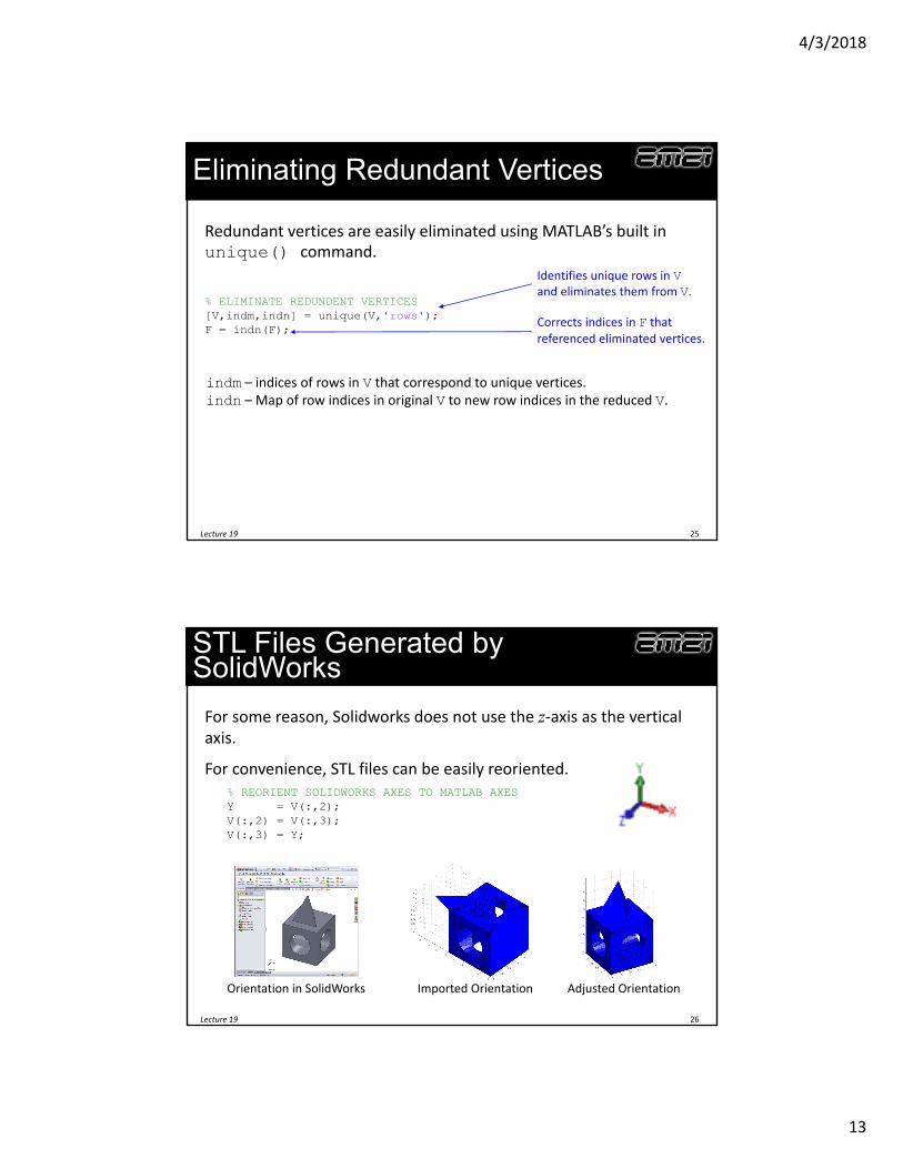
For some reason, Solidworks does not use the z‐axis as the vertical axis.
For convenience, STL files can be easily reoriented.% REORIENT SOLIDWORKS AXES TO MATLAB AXESY = V(:,2);V(:,2) = V(:,3);V(:,3) = Y;
Orientation in SolidWorks Imported Orientation Adjusted Orientation

4/3/2018
14
Visualizing Surface Meshes
in MATLAB
How to Draw the Object
Lecture 19 28
Given the faces and vertices, the object can be drawn in MATLAB using the patch() command.
% DRAW STRUCTURE USING PATCHESP = patch('faces',F,'vertices',V);set(P,'FaceColor','b','FaceAlpha',0.5); set(P,'EdgeColor','k','LineWidth',2);

4/3/2018
15
Generating Faces and
Vertices Using MATLAB
MATLAB Surfaces
Lecture 19 30
Surfaces composed of square facets are stored in X, Y, and Z arrays.
The surface shown is constructed of arrays that are all 5×5.

4/3/2018
16
Direct Construction of the Surface Mesh
Lecture 19 31
% CREATE A UNIT SPHERE[X,Y,Z] = sphere(41);
MATLAB has a number of built‐in commands for generating surfaces. Some of these are cylinder(), sphere() and ellipsoid().
Surfaces can be converted to triangular patches (facets and vertices) using the surf2patch() function.
% CONVERT TO PATCH[F,V] = surf2patch(X,Y,Z,’triangles’);
The faces and vertices can be directly visualized using the patch()function.
% VISUALIZE FACES AND VERTICESh = patch('faces',F,'vertices',V);set(h,'FaceColor',[0.5 0.5 0.8],'EdgeColor','k');
Grid Surface Mesh
Lecture 19 32
% CREATE ELLIPTICAL OBJECTOBJ = (X/rx).^2 + (Y/ry).^2 + (Z/rz).^2;OBJ = (OBJ < 1);
% CREATE SURFACE MESH[F,V] = isosurface(X,Y,Z,OBJ,0.5);
3D objects on a grid can be converted to a surface mesh using the command isosurface().
Object on 3D Grid Surface Mesh

4/3/2018
17
May Need isocaps()
Lecture 19 33
When 3D objects extend to the edge of the grid, you may need to use isocaps() in addition to isosurface().
isosurface() isocaps() isosurface()+ isocaps()
% CREATE SURFACE MESH[F,V] = isosurface(X,Y,Z,OBJ,0.5);[F2,V2] = isocaps(X,Y,Z,OBJ,0.5);
Combining Faces and Vertices from Two Objects
Lecture 19 34
There are no functions in MATLAB to perform Boolean operations on multiple meshes. We can, however, combine the faces and vertices from two objects. Be careful this does not result in overlaps or gaps between objects.
F1 and V1 F2 and V2CorrectlyCombined
% COMBINE FACES AND VERTICESF3 = [ F1 ; F2+length(V1(:,1)) ]V3 = [ V1 ; V2 ]
IncorrectlyCombined
% WRONG WAY TO % COMBINE FACES AND VERTICESF3 = [ F1 ; F2 ]V3 = [ V1 ; V2 ]

4/3/2018
18
Converting Surface Meshes to Objects on a
3D Grid
Example – Pyramid
Lecture 19 36
SolidWorks Model
Import STL into MATLAB Convert to Volume Object
ER(nx,ny,nz)

4/3/2018
19
Example – Dinosaur
Lecture 19 37
Import STL into MATLAB Convert to Volume Object
ER(nx,ny,nz)
Lecture 19 38
MATLAB Functions for “Voxelization” of STL Files
The Mathworks website has excellent functions for converting surface meshes to points on a 3D array.
Function for Voxelizationhttp://www.mathworks.com/matlabcentral/fileexchange/27390‐mesh‐voxelisation

4/3/2018
20
Converting Images and 2D Objects to STL
Load and Resize the Image
Lecture 19 40
% LOAD IMAGEB = imread(‘letter.jpg');
% RESIZE IMAGEB = imresize(B,0.2);[Nx,Ny,Nc] = size(B);
This will give us a coarser mesh in order to be faster and more memory efficient.

4/3/2018
21
Flatten the Image
Lecture 19 41
% FLATTEN COLOR IMAGEB = double(B);B = B(:,:,1) + B(:,:,2) + B(:,:,3);B = 1 - B/765;
Images loaded from file usually contain RGB information making them 3D arrays. These arrays must be converted to flat 2D arrays before meshing.
Stack the Image
Lecture 19 42
% STACK IMAGEB(:,:,2) = B;
We will mesh the image using isocaps(), but that function requires a 3D array. So, we will stack this image to be two layers thick.

4/3/2018
22
Mesh the Image Using isocaps()
Lecture 19 43
% CREATE 2D MESH[F,V] = isocaps(ya,xa,[0 1],B,0.5,'zmin');
We only wish to mesh a single surface so we give isocaps() the additional input argument ‘zmin’ to do this.
Save the Mesh as an STL File
Lecture 19 44
We can save this mesh as an STL file.

4/3/2018
23
Extrude Using Blender (1 of 2)
Lecture 19 45
1. Open Blender.exe.2. File Import Stl (.stl)3. Open the STL file you just created.
Extrude Using Blender (2 of 2)
Lecture 19 46
1. Select the object with right mouse click.
2. Press TAB to enter Edit mode.3. Press ‘e’ to extrude mesh.4. Press TAB again to exit Edit mode.5. You can now edit your object
or export as a new 3D STL file.

4/3/2018
24
Point Clouds
What is a Point Cloud?
Lecture 19 48
Klein Bottle (see MATLAB demos) Point Cloud Description of a Klein Bottle
Point clouds represent the outside surface of object as a set of vertices defined by X, Y, and Z coordinates. They are typically generated by 3D scanners, but can also be used to export 3D objects from MATLAB into SolidWorks or other CAD programs.

4/3/2018
25
Other Examples of Point Clouds
Lecture 19 49
Point Cloud Data
Lecture 19 50
The position of all the points in the point cloud can be stored in an array.
PC =0.1200 0.0000 0.70710.1159 -0.0311 0.70710.0311 -0.1159 0.70710.0000 -0.1200 0.7071-0.0311 -0.1159 0.7071-0.0600 -0.1039 0.7071
1 1 1
2 2 2
3 3 3PC
N N N
x y z
x y z
x y z
x y z

4/3/2018
26
Saving Point Cloud Data to File (1 of 2)
Lecture 19 51
Point cloud data files are comma separated text files with the extension “.xyz”
These can be easily generated using the built‐in MATLAB command csvwrite().
% SAVE POINT CLOUD AS A COMMA SEPERATED FILEPC = [ X Z Y ];dlmwrite('pointcloud.xyz',PC,'delimiter',',','newline','pc');
PC = [ X Z Y ];PC = [ X Y Z ];
Saving Point Cloud Data to File (2 of 2)
Lecture 19 52
SolidWorks wants to see an X Y Z at the start of the file.
You can add this manually using Notepad or write a more sophisticated MATLAB text file creator.

4/3/2018
27
Activate ScanTo3D Add-In in SolidWorks
Lecture 19 53
First, you will need to activate the ScanTo3D in SolidWorks.
Click ToolsAdd‐Ins.
Check the Scanto3D check box.
Click OK.
Open the Point Cloud File
Lecture 19 54

4/3/2018
28
Run the Mesh Prep Wizard
Lecture 19 55
ToolsScanTo3DMesh Prep Wizard…1. Run the Mesh Prep Wizard.2. Select the point cloud.3. Click the right array button.4. Orientation method, select None
because we did this in MATLAB.5. Noise removal, zero assuming
geometry came from MATLAB.6. Work through all options.7. Click the green check mark to finish.
Point Cloud Density
Lecture 19 56

4/3/2018
29
Final Notes on Point Clouds
• Other CAD packages have better point cloud import capabilities than SolidWorks. Rhino 3D is said to be excellent.
• Generating a solid model from the data can be done in SolidWorks. The meshed model is essentially used as a template for creating the solid model. This procedure is beyond the scope of this lecture.
Lecture 19 57
Importing Custom
Polygons into SolidWorks

4/3/2018
30
The Problem
Lecture 19 59
Suppose we calculate the vertices of a polygon from an optimization in MATLAB.
How do we important the vertices so that the polygon can be imported exactly into Solidworks so that it can be extruded, cut, modified, etc.?
There is no feature in SolidWorks to do this!!
Example Application
Lecture 19 60
Placing a GMR filter onto a curved surface.
Grating period is spatially varied to compensate.
1inc
0 0 inc inc
0
sintan
1 cos
sin
1 cos cos
cos cos
x
r
r
x Rxx
R d R x R
K x K k n x
x K x dx
x fx
x f
R. C. Rumpf, M. Gates, C. L. Kozikowski, W. A. Davis, "Guided‐Mode Resonance Filter Compensated to Operate on a Curved Surface," PIER C, Vol. 40, pp. 93‐103, 2013.

4/3/2018
31
Be Careful About XYZ Curves
Lecture 19 61
There is a feature in SolidWorks “Curve Through XYZ Points” that appears to import discrete points, but it fits the points to a spline. This effectively rounds any corners and may produce intersections that cannot be rendered.
This should be a square! The four points are fit to a spline!
Step 1 – Define the Polygon
Lecture 19 62
Create an N×3 array in memory which contains all of the points around the perimeter of the polygon. N is the number of points.
P =0.6448 0 01.0941 0.3758 01.3427 1.0452 00.3642 0.5573 00.4753 1.8765 0
-0.0651 0.7853 0-0.5258 1.1984 0-0.4824 0.5240 0-0.8912 0.4822 0-0.9966 0.1664 0-0.9087 -0.1517 0-1.0666 -0.5774 0-1.1762 -1.2777 0-0.5403 -1.2314 0-0.1403 -1.6931 00.3818 -1.5074 00.7795 -1.1927 00.8293 -0.6455 01.0972 -0.3766 00.6448 -0.0000 0

4/3/2018
32
Step 2 – Save as an IGES from MATLAB
Lecture 19 63
There is a function called igesout() available for free download from the Mathworks website. This will save your polygon to an IGES file.
% SAVE IGES FILEigesout(P,'poly');
This creates a file called “poly.igs” in your working directory.
Step 3 – Open the IGES in SolidWorks (1 of 2)
Lecture 19 64
Select the IGES file type in the [Open] file dialog. Then click on the [Options…] button.

4/3/2018
33
Step 3 – Open the IGES in SolidWorks (2 of 2)
Lecture 19 65
1.Make sure that “Surface/solid entities” is unchecked
2. Ensure that “Free point/curve entities” is checked.
3.Click on the “Import as sketch(es) radio button.
Open the file.
Step 4 – Convert to a Standard 2D Sketch
Lecture 19 66
The polygon imports as a 3D sketch by default.
Edit the 3D sketch and copy.
Open a new 2D sketch and paste.
Now you can do whatever you wish with the sketch! Extrude, revolve, cut extrude, etc.

4/3/2018
34
STL to CAD Conversion
Import STL Into MeshLab
Lecture 19 68
1. Open meshlab.exe.2. File Import Mesh3. Open the 3D STL file you just created.

4/3/2018
35
Convert to SolidWorks Part
Lecture 19 69
1. Open meshlab.exe.2. File Export Mesh As3. Select DXF file type.4. Save mesh.5. Launch SolidWorks.6. File Open7. Select DXF file.8. Select ‘Import to a new part as:’
then ‘3D curves or model’ then ‘Next >.’
9. Select ‘All Layers’