Lecture 19

aCGH and Microarray Data Analysis

Introduction to Bioinformatics

CENTR

FORINTEGRATIVE

BIOINFORMATICSVU

E

A.s. donderdag 22 meiPracticum in S3.29 en S3.53

(niet S.3.45)

Introduction to Bioinformatics

CENTR

FORINTEGRATIVE

BIOINFORMATICSVU

E

Array-CGH (Comparative Genomics Hybridisation)

• New microarray-based method to determine local chromosomal copy numbers

• Gives an idea how often pieces of DNA are copied

• This is very important for studying cancers, which have been shown to often correlate with copy events!

• Also referred to as ‘a-CGH’

Tumor Cell

Chromosomes of tumor cell:

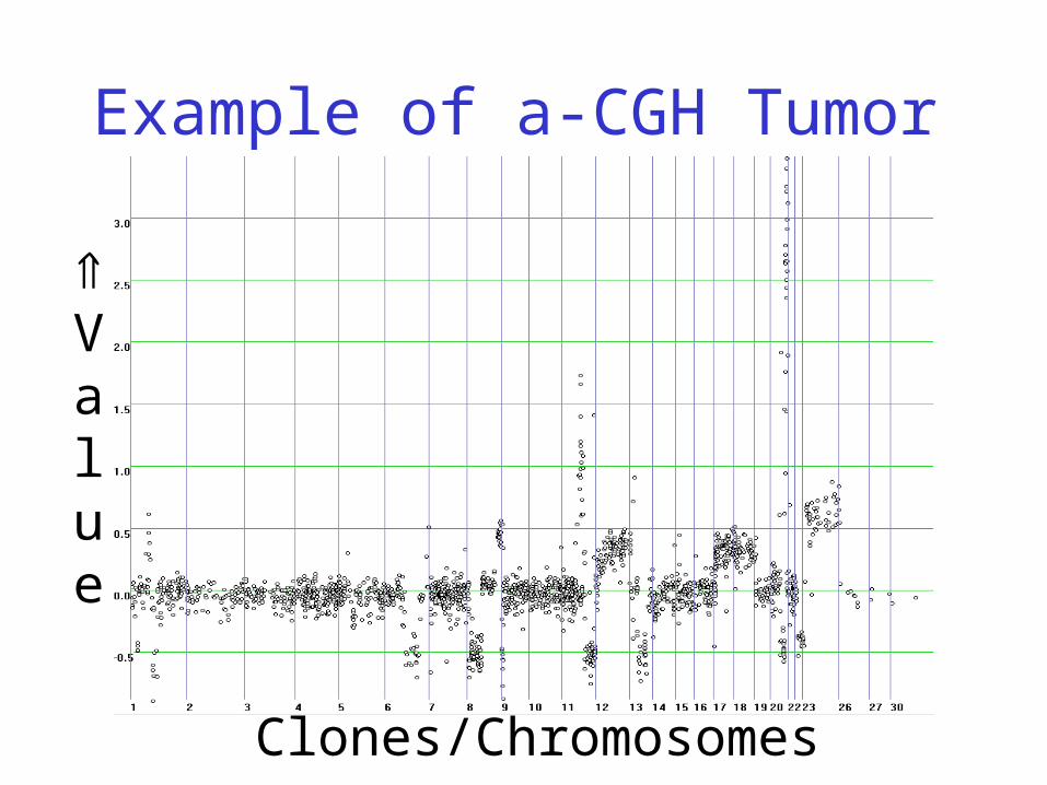
Example of a-CGH Tumor

Clones/Chromosomes

Value

a-CGH vs. Expression

a-CGH• DNA

– In Nucleus

– Same for every cell

• DNA on slide• Measure Copy

Number Variation

Expression• RNA

– In Cytoplasm

– Different per cell

• cDNA on slide• Measure Gene

Expression

CGH Data

Clones/Chromosomes

Copy#

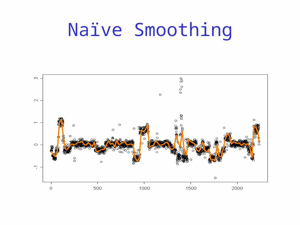
Naïve Smoothing

“Discrete” Smoothing

Copy numbers are integers

Question: how do we best break up the dataset in same-copy number regions (with breakpoints in between)?

Why Smoothing ?• Noise reduction

• Detection of Loss, Normal, Gain, Amplification

• Breakpoint analysis

Recurrent (over tumors) aberrations may indicate:–an oncogene or –a tumor suppressor gene

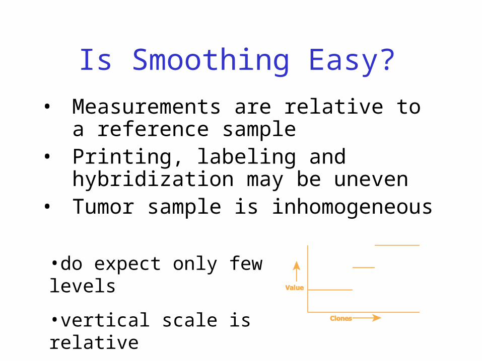
Is Smoothing Easy?

• Measurements are relative to a reference sample

• Printing, labeling and hybridization may be uneven

• Tumor sample is inhomogeneous

•do expect only few levels

•vertical scale is relative

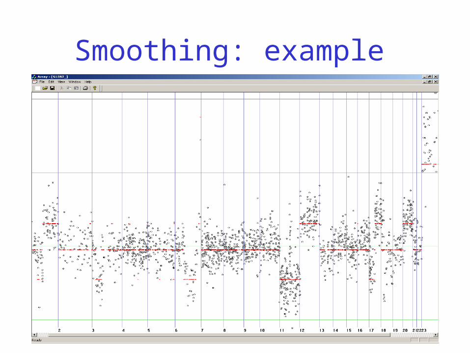
Smoothing: example

Problem Formalization

A smoothing can be described by• a number of breakpoints • corresponding levels

A fitness function scores each smoothing according to fitness to the data

An algorithm finds the smoothing with the highest fitness score.

Breakpoint Detection

• Identify possibly damaged genes:– These genes will not be expressed anymore

• Identify recurrent breakpoint locations:– Indicates fragile pieces of the chromosome

• Accuracy is important:– Important genes may be located in a region

with (recurrent) breakpoints

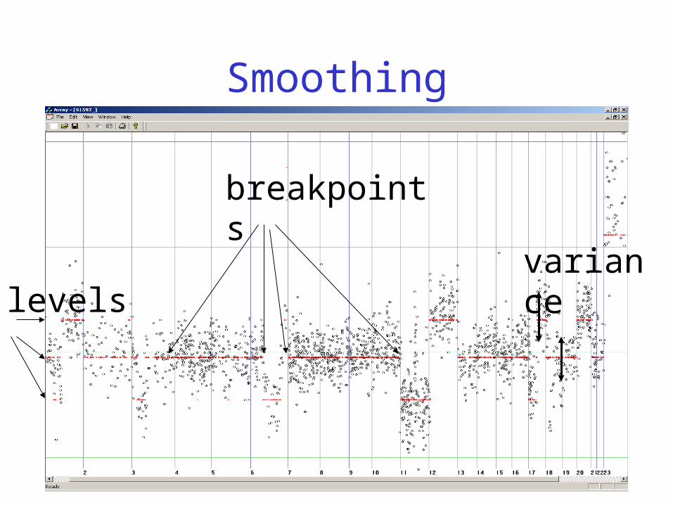
Smoothing

breakpoints

levelsvariance

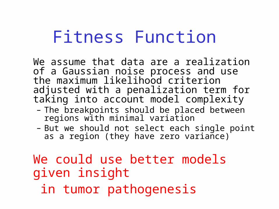
Fitness Function We assume that data are a realization of a

Gaussian noise process and use the maximum likelihood criterion adjusted with a penalization term for taking into account model complexity– The breakpoints should be placed between regions with

minimal variation– But we should not select each single point as a region

(they have zero variance)

We could use better models given insight in tumor pathogenesis

Fitness Function (2)CGH values: x1 , ... , xn

breakpoints: 0 < y1 … yN xN

levels:

error variances:

likelihood of each discrete region:

Fitness Function (3)

Maximum likelihood estimators of μ and 2 can be found explicitly

Need to add a penalty to log likelihood tocontrol number N of breakpoints, in order to avoid too many breakpoints

penalty

Comparison to Expert

expert

algorithm

aCGH data after smoothingPatient Clone 1 Clone 2 Clone 3 Clone 4 Clone 5 Clone 6

1 5 6 18 110 -2 10

2 7 6 3 98 -1 11

3 18 17 24 75 0 8

REF 5 6 35 62 -1 9

Patient Clone 1 Clone 2 Clone 3 Clone 4 Clone 5 Clone 6

1 0 0 -1 1 -1 0

2 0 0 -1 1 0 0

3 1 1 0 0 0 0

REF 0 6 0 0 0 0

Often, gain, no-difference and loss are indicated by 1, 0 and -1 respectively

aCGH Summary

• Chromosomal gains and losses tell about diseases• Need (discrete) smoothing (breakpoint

assignment) of data• Problem: large variation between patients• Identify consistent gains and losses and relate

those to a given cancer type• Chances for treatment and drugs• Important question: what do gained or lost

fragments do and how do they relate to disease?

Analysing microarray expression profiles

Some statistical research stimulated by microarray data analysis

•Experimental design : Churchill & Kerr

•Image analysis: Zuzan & West, ….

•Data visualization: Carr et al

•Estimation: Ideker et al, ….

•Multiple testing: Westfall & Young , Storey, ….

•Discriminant analysis: Golub et al,…

•Clustering: Hastie & Tibshirani, Van der Laan, Fridlyand & Dudoit, ….

•Empirical Bayes: Efron et al, Newton et al,…. Multiplicative models: Li &Wong

•Multivariate analysis: Alter et al

•Genetic networks: D’Haeseleer et al and more

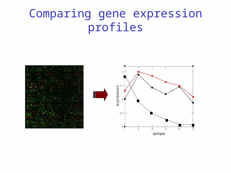
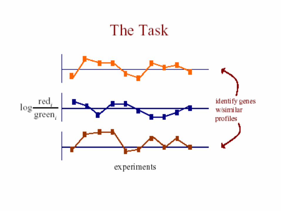
Comparing gene expression profiles

Normalising microarray data (z-scores)

•z = (xi - )/, where is mean and is standard deviation of a series of measurements x1 .. xn. This leads to normalised z-scores (measurements) with zero mean (=0) and unit standard deviation (=1)

•If M normally distributed, then probability that z lies outside range -1.96 < z < 1.96 is 5%

•There is evidence that log(R/G) ration are normally distributed. Therefore, R/G is said to be log-normally distributed

The Data• each measurement represents

Log(Redi/Greeni)

where red is the test expression level, and green isthe reference level for gene G in the i th experiment

• the expression profile of a gene is the vector of

measurements across all experiments [G1 .. Gn]

The Data

• m genes measured in n experiments:

g1,1 ……… g1,n

g2,1 ………. g2,n

gm,1 ………. gm,n Vector for 1 gene

29

Which similarity or dissimilarity measure?

• A metric is a measure of the similarity or dissimilarity between two data objects

• Two main classes of metric:– Correlation coefficients (similarity)

• Compares shape of expression curves• Types of correlation:

– Centered.– Un-centered.– Rank-correlation

– Distance metrics (dissimilarity)• City Block (Manhattan) distance• Euclidean distance

30

• Pearson Correlation Coefficient (centered correlation)

Sx = Standard deviation of x

Sy = Standard deviation of y

n

i y

i

x

in S

yy

S

xx

11

1

Correlation (a measure between -1 and 1)

Positive correlation Negative correlation

You can use absolute correlation to capture both positive and negative correlation

31

Potential pitfalls

Correlation = 1

32

Distance metrics• City Block (Manhattan)

distance:– Sum of differences across

dimensions

– Less sensitive to outliers

– Diamond shaped clusters

• Euclidean distance:– Most commonly used distance

– Sphere shaped cluster

– Corresponds to the geometric distance into the multidimensional space

i

ii yxYXd ),( i

ii yxYXd 2)(),(

where gene X = (x1,…,xn) and gene Y=(y1,…,yn)

X

Y

Condition 1

Co

nd

itio

n 2

Condition 1

X

Y

Co

nd

itio

n 2

33

Euclidean vs Correlation (I)• Euclidean distance

• Correlation

Euclidean

Correleation

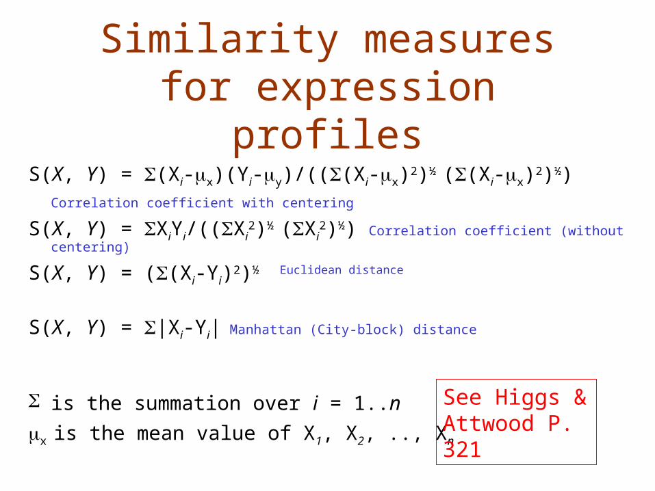
Similarity measures for expression profiles

S(X, Y) = (Xi-x)(Yi-y)/(((Xi-x)2)½ ((Xi-x)2)½)Correlation coefficient with centering

S(X, Y) = XiYi/((Xi2)½ (Xi

2)½) Correlation coefficient (without centering)

S(X, Y) = ((Xi-Yi)2)½ Euclidean distance

S(X, Y) = |Xi-Yi|Manhattan (City-block) distance

is the summation over i = 1..n

x is the mean value of X1, X2, .., Xn

See Higgs & Attwood P. 321

35

Classification Using Gene Expression Data

Three main types of problems associated with tumor classification:

• Identification of new/unknown tumor classes using gene expression profiles (unsupervised learning – clustering)

• Classification of malignancies into known classes (supervised learning – discrimination)

• Identification of “marker” genes that characterize the different tumor classes (feature or variable selection).

Partitional Clustering

• divide instances into disjoint clusters (non-overlapping groups of genes)

– flat vs. tree structure

• key issues

– how many clusters should there be?

– how should clusters be represented?

Partitional Clustering from aHierarchical Clustering

we can always generate a partitional clustering from ahierarchical clustering by “cutting” the tree at some level

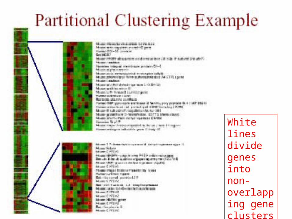
White lines divide genes into non-overlapping gene clusters

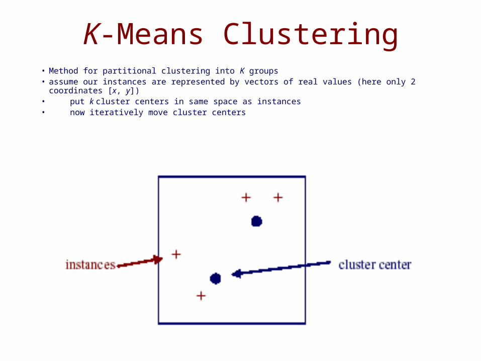
K-Means Clustering• Method for partitional clustering into K groups• assume our instances are represented by vectors of real values (here only 2 coordinates [x, y])• put k cluster centers in same space as instances• now iteratively move cluster centers

K-Means Clustering• each iteration involves two steps:

– assignment of instances to clusters– re-computation of the means

41

Supervised Learning

Train dataset

ML algorithm

model predictionnew observation

System (unknown)observationsproperty of interest

?

supervisor

Classification

42

Unsupervised Learning

ML for unsupervised learning attempts to discover interesting structure in the available data

Data mining, Clustering

43

What is your question?• What are the targets genes for my knock-out gene?• Look for genes that have different time profiles between different cell types.

Gene discovery, differential expression

• Is a specified group of genes all up-regulated in a specified conditions?Gene set, differential expression

• Can I use the expression profile of cancer patients to predict survival?• Identification of groups of genes that are predictive of a particular class of tumors?

Class prediction, classification

• Are there tumor sub-types not previously identified? • Are there groups of co-expressed genes?

Class discovery, clustering

• Detection of gene regulatory mechanisms. • Do my genes group into previously undiscovered pathways?

Clustering. Often expression data alone is not enough, need to incorporate functional and other information

44

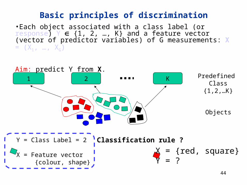
Predefined Class

{1,2,…K}

1 2 K

Objects

Basic principles of discrimination•Each object associated with a class label (or response) Y {1, 2, …, K} and a feature vector (vector of predictor variables) of G measurements: X = (X1, …, XG)

Aim: predict Y from X.

X = {red, square} Y = ?

Y = Class Label = 2

X = Feature vector {colour, shape}

Classification rule ?

45

Discrimination and PredictionLearning Set

Data with known classes

ClassificationTechnique

Classificationrule

Data with unknown classes

ClassAssignment

Discrimination

Prediction

46

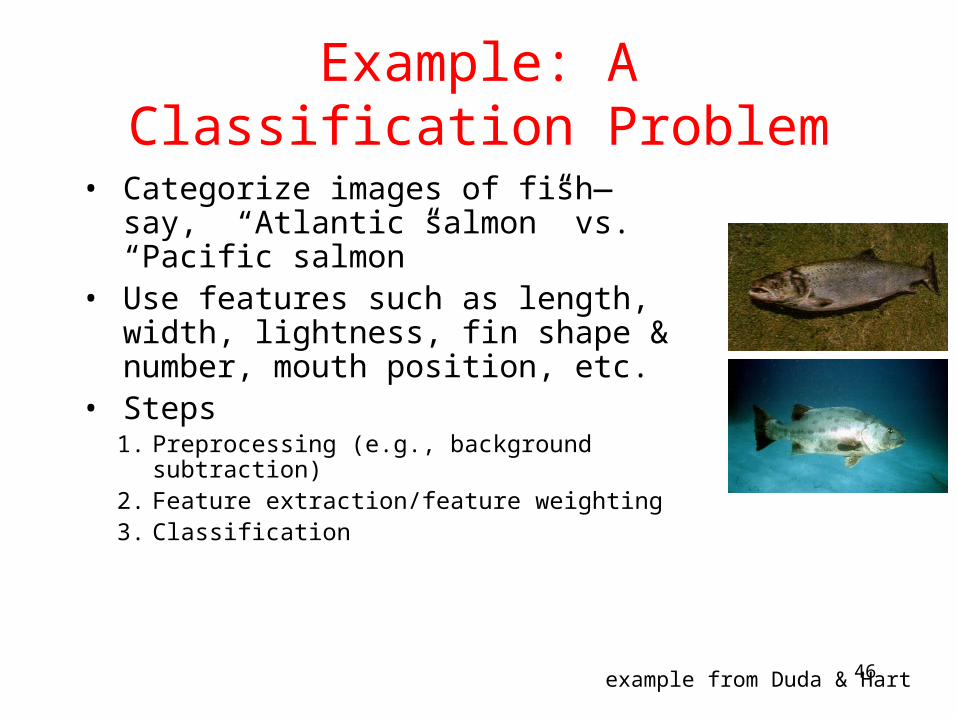
Example: A Classification Problem

• Categorize images of fish—say, “Atlantic salmon” vs. “Pacific salmon”

• Use features such as length, width, lightness, fin shape & number, mouth position, etc.

• Steps1. Preprocessing (e.g., background subtraction)2. Feature extraction/feature weighting3. Classification

example from Duda & Hart

47

Classification in Bioinformatics

• Computational diagnostic: early cancer detection

• Tumor biomarker discovery

• Protein structure prediction (threading)

• Protein-protein binding sites prediction

• Gene function prediction

• …

Example 1Breast tumor classification

van 't Veer et al (2002) Nature 415, 530

Dutch Cancer Institute (NKI)

Prediction of clinical outcome of breast cancer

DNA microarray experiment117 patients25000 genes

49

?Bad prognosis

recurrence < 5yrsGood Prognosis

recurrence > 5yrs

ReferenceL van’t Veer et al (2002) Gene expression profiling predicts clinical outcome of breast cancer. Nature, Jan..

ObjectsArray

Feature vectorsGene

expression

Predefine classesClinicaloutcome

new array

Learning set

Classificationrule

Good Prognosisrecurrence > 5 yrs

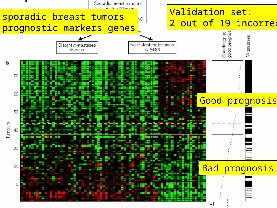
78 sporadic breast tumors70 prognostic markers genes

Good prognosis

Bad prognosis

Validation set:2 out of 19 incorrect

Is there work to do on van 't Veer et al. data ?• What is the minimum number of genes required in

these classification models (to avoid chance classification)

• What is the maximum number of genes (avoid overfitting)

• What is the relation to the number of samples that must be measured?

• Rule of thumb: minimal number of events per variable (EPV)>10– NKI study ~35 tumors (events) in each group 35/10=3.5

genes should maximally have been selected (70 were selected in the breast cancer study) overfitting? Is the classification model adequate?

53

Classification Techniques

• K Nearest Neighbor classifier

• Support Vector Machines

• …

54

Instance Based Learning (IBL)Key idea: just store all training examples <xi,f(xi)>

Nearest neighbor:• Given query instance xq, first locate nearest training

example xn, then estimate f(xq)=f(xn)

K-nearest neighbor:

• Given xq, take vote among its k nearest neighbors (if discrete-valued target function)

• Take mean of values of k nearest neighbors (if real-

valued) f(xq)=i=1k f(xi)/k

55

K-Nearest Neighbor• The k-nearest neighbor algorithm is amongst the simplest of

all machine learning algorithms.

• An object is classified by a majority vote of its neighbors, with the object being assigned to the class most common amongst its k nearest neighbors.

• k is a positive integer, typically small. If k = 1, then the object is simply assigned to the class of its nearest neighbor.

• K-NN can do multiple class prediction (more than two cancer subtypes, etc.)

• In binary (two class) classification problems, it is helpful to choose k to be an odd number as this avoids tied votes.

Adapted from Wikipedia

56

K-Nearest Neighbor• A lazy learner …

• Issues: – How many neighbors?– What similarity measure?

Example of k-NN classification. The test sample (green circle) should be classified either to the first class of blue squares or to the second class of red triangles. If k = 3 it is classified to the second class because there are 2 triangles and only 1 square inside the inner circle. If k = 5 it is classified to first class (3 squares vs. 2 triangles inside the outer circle).

From Wikipedia

57

When to Consider Nearest Neighbors

• Instances map to points in RN

• Less than 20 attributes per instance• Lots of training data

Advantages:• Training is very fast • Learn complex target functions• Do not loose information

Disadvantages:• Slow at query time • Easily fooled by irrelevant attributes

Voronoi Diagrams• Voronoi diagrams partition a space with objects in the

same way as happens when you throw a number of pebbles in water -- you get concentric circles that will start touching and by doing so delineate the area for each pebble (object).

• The area assigned to each object can now be used for weighting purposes

• A nice example from sequence analysis is by Sibbald, Vingron and Argos (1990)Sibbald, P. and Argos, P. 1990. Weighting aligned protein or nucleic acid sequences to correct for unequal representation. JMB 216:813-818.

59

Voronoi Diagram

query point qf

nearest neighbor qi

60

3-Nearest Neighbors

query point qf

3 nearest neighbors

2x,1o

Can use Voronoi areas for weighting

61

7-Nearest Neighbors

query point qf

7 nearest neighbors

3x,4o

62

k-Nearest Neighbors• The best choice of k depends upon the data; generally,

larger values of k reduce the effect of noise on the classification, but make boundaries between classes less distinct.

• A good k can be selected by various heuristic techniques, for example, cross-validation. If k = 1, the algorithm is called the nearest neighbor algorithm.

• The accuracy of the k-NN algorithm can be severely degraded by the presence of noisy or irrelevant features, or if the feature scales are not consistent with their importance.

• Much research effort has been put into selecting or scaling features to improve classification, e.g. using evolutionary algorithms to optimize feature scaling.

The curse of dimensionality

• Term introduced by Richard Bellman1

• Problems caused by the exponential increase in volume associated with adding extra dimensions to a (mathematical) space.

• So: the ‘problem space’ increases with the number of variables/features.

1Bellman, R.E. 1957. Dynamic Programming. Princeton University Press, Princeton, NJ

64

Example: Tumor Classification

• Reliable and precise classification essential for successful cancer treatment

• Current methods for classifying human malignancies rely on a variety of morphological, clinical and molecular variables

• Uncertainties in diagnosis remain; likely that existing classes are heterogeneous

• Characterize molecular variations among tumors by monitoring gene expression (microarray)

• Hope: that microarrays will lead to more reliable tumor classification (and therefore more appropriate treatments and better outcomes)

65

Tumor Classification Using Gene Expression Data

Three main types of ML problems associated with tumor classification:

• Identification of new/unknown tumor classes using gene expression profiles (unsupervised learning – clustering)

• Classification of malignancies into known classes (supervised learning – discrimination)

• Identification of “marker” genes that characterize the different tumor classes (feature or variable selection).

66

Example Leukemia experiments (Golub et al 1999)

Goal. To identify genes which are differentially expressed in acute lymphoblastic leukemia (ALL) tumours in comparison with acute myeloid leukemia (AML) tumours.

• 38 tumour samples: 27 ALL, 11 AML.• Data from Affymetrix chips, some pre-processing.• Originally 6,817 genes; 3,051 after reduction.

Data therefore 3,051 38 array of expression values.

Acute lymphoblastic leukemia (ALL) is the most common malignancy in children 2-5 years in age, representing nearly one third of all pediatric cancers.

Acute Myeloid Leukemia (AML) is the most common form of myeloid leukemia in adults (chronic lymphocytic leukemia is the most common form of leukemia in adults overall). In contrast, acute myeloid leukemia is an uncommon variant of leukemia in children. The median age at diagnosis of acute myeloid leukemia is 65 years of age.

67

B-ALL T-ALL AML

ReferenceGolub et al (1999) Molecular classification of cancer: class discovery and class prediction by gene expression monitoring. Science 286(5439): 531-537.

ObjectsArray

Feature vectorsGene

expression

Predefine classes

Tumor type

?

new array

Learning set

ClassificationRule

T-ALL

68

Nearest neighbor rule

69

SVM• SVMs were originally proposed by Boser, Guyon and Vapnik in

1992 and gained increasing popularity in late 1990s.

• SVMs are currently among the best performers for a number of classification tasks ranging from text to genomic data.

• SVM techniques have been extended to a number of tasks such as regression [Vapnik et al. ’97], principal component analysis [Schölkopf et al. ’99], etc.

• Most popular optimization algorithms for SVMs are SMO [Platt ’99] and SVMlight

[Joachims’ 99], both use decomposition to hill-climb over a subset of αi’s at a time.

• Tuning SVMs remains a black art: selecting a specific kernel and parameters is usually done in a try-and-see manner.

70

SVM

• In order to discriminate between two classes, given a training dataset– Map the data to a higher dimension space

(feature space)

– Separate the two classes using an optimal linear separator

71

Feature Space Mapping• Map the original data to some higher-dimensional

feature space where the training set is linearly separable:

Φ: x → φ(x)

72

The “Kernel Trick”• The linear classifier relies on inner product between vectors K(xi,xj)=xi

Txj

• If every datapoint is mapped into high-dimensional space via some transformation Φ: x → φ(x), the inner product becomes:

K(xi,xj)= φ(xi) Tφ(xj)

• A kernel function is some function that corresponds to an inner product in some expanded feature space.

• Example:

2-dimensional vectors x=[x1 x2]; let K(xi,xj)=(1 + xiTxj)2

,

Need to show that K(xi,xj)= φ(xi) Tφ(xj):

K(xi,xj)=(1 + xiTxj)2

,= 1+ xi12xj1

2 + 2 xi1xj1 xi2xj2+ xi2

2xj22 + 2xi1xj1 + 2xi2xj2=

= [1 xi12 √2 xi1xi2 xi2

2 √2xi1 √2xi2]T [1 xj12 √2 xj1xj2 xj2

2 √2xj1 √2xj2] =

= φ(xi) Tφ(xj), where φ(x) = [1 x1

2 √2 x1x2 x22 √2x1 √2x2]

73

Linear Separators

Which one is the best?

74

Optimal hyperplane

ρ

Support vector

margin

Optimal hyper-plane

Support vectors uniquely characterize optimal hyper-plane

75

Optimal hyperplane: geometric view

11

11

ii

ii

yforbxw

yforbxw The first class

The second class

76

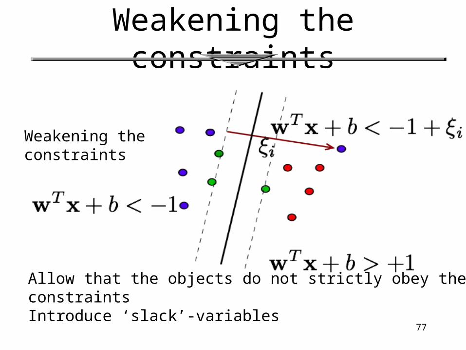
Soft Margin Classification • What if the training set is not linearly separable?

• Slack variables ξi can be added to allow misclassification of difficult or noisy examples.

ξjξk

77

Weakening the constraints

Weakening the constraints

Allow that the objects do not strictly obey the constraintsIntroduce ‘slack’-variables

78

SVM

• Advantages:– maximize the margin between two classes in the feature

space characterized by a kernel function

– are robust with respect to high input dimension

• Disadvantages:– difficult to incorporate background knowledge

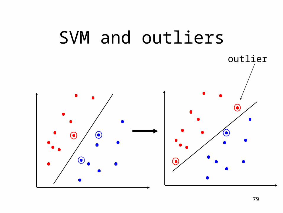
– Sensitive to outliers

79

SVM and outliersoutlier

80

Classifying new examples

• Given new point x, its class membership is

sign[f(x, *, b*)], where ***

1

***** ),,( bybybbfSVi iii

N

i iii xxxxxwx

Data enters only in the form of dot products!

**** ),(),,( bKybfSVi iii

xxx

and in general

Kernel function

What is feature selection?

• Reducing the feature space by removing some of the (non-relevant) features.

• Also known as:– variable selection– feature reduction– attribute selection– variable subset selection

• It is cheaper to measure less variables.

• The resulting classifier is simpler and potentially faster.

• Prediction accuracy may improve by discarding irrelevant variables.

• Identifying relevant variables gives more insight into the nature of the corresponding classification problem (biomarker detection).

• Alleviate the “curse of dimensionality”.

Why select features?

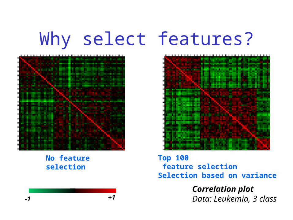
Correlation plotData: Leukemia, 3 class

No feature selection

Top 100 feature selectionSelection based on variance

-1 +1

Why select features?

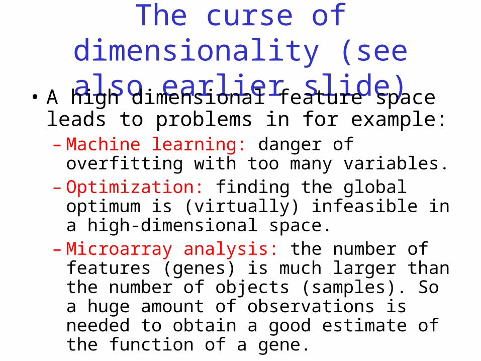
The curse of dimensionality (see also earlier slide)

• A high dimensional feature space leads to problems in for example:– Machine learning: danger of overfitting with too

many variables.– Optimization: finding the global optimum is

(virtually) infeasible in a high-dimensional space.– Microarray analysis: the number of features

(genes) is much larger than the number of objects (samples). So a huge amount of observations is needed to obtain a good estimate of the function of a gene.

• Few samples for analysis (38 labeled).

• Extremely high-dimensional data (7129 gene expression values per sample).

• Noisy data.

• Complex underlying mechanisms, not fully understood.

Microarray Data Challenges to Machine Learning Algorithms:

Some genes are more useful than others for building classification models

Example: genes 36569_at and 36495_at are useful

Example: genes 36569_at and 36495_at are useful

AML

ALL

Some genes are more useful than others for building classification models

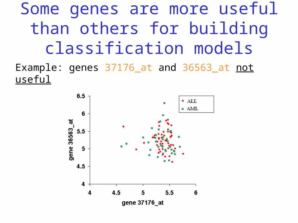
Example: genes 37176_at and 36563_at not useful

Some genes are more useful than others for building classification models

Importance of feature (gene) selection

• Majority of genes are not directly related to leukemia.

• Having a large number of features enhances the model’s flexibility, but makes it prone to overfitting.

• Noise and the small number of training samples makes this even more likely.

• Some types of models, like kNN do not scale well with many features.

1. Distance metrics to capture class separation.

2. Rank genes according to distance metric score.

3. Choose the top n ranked genes.

HIGH score LOW score

How do we choose the most relevant of the 7219 genes?

Classical exampleGenome-Wide Cluster Analysis

Eisen dataset (a classic)• Eisen et al., PNAS 1998• S. cerevisiae (baker’s yeast)

– all genes (~ 6200) on a single array– measured during several processes

• human fibroblasts– 8600 human transcripts on array– measured at 12 time points during serum stimulation

The Eisen Data

• 79 measurements for yeast data• collected at various time points during– diauxic shift (shutting down genes for

metabolizing sugars, activating those for metabolizing ethanol)

– mitotic cell division cycle– sporulation– temperature shock– reducing shock

Eisen et al. cDNA array results

• redundant representations of genes cluster together– but individual genes can be distinguished from

related genes by subtle differences in expression

• genes of similar function cluster together– e.g. 126 genes were observed to be strongly

down-regulated in response to stress

Eisen et al. Results

• 126 genes down-regulated in response to stress

– 112 of these 126 genes encode ribosomal and other proteins related to translation

– agrees with previously known result that yeast responds to favorable growth conditions by increasing the production of ribosomes