Lecture 18 Wind and Turbulence Part 3 Surface Boundary … · Biometeorology, ESPM 129 2 Thom...

Biometeorology, ESPM 129

1

Lecture 18, Wind and Turbulence, Part 3, Surface Boundary Layer: Theory and Principles, Cont Instructor: Dennis Baldocchi Professor of Biometeorology Ecosystem Science Division Department of Environmental Science, Policy and Management 345 Hilgard Hall University of California, Berkeley Berkeley, CA 94720 October 17, 2014 Topics to be Covered A. Variations in Space, cont. 1.Wind over Tall Vegetation

a. Zero plane displacement and Roughness Length i. Variations of zo and d with LAI b. Role of stability on wind profiles

c. Monin Obuhkov theory; Richardson number 2. Wind over hills 3 Eddy Exchange Coefficients, Influence of Scalar, Stability and Roughness Sublayer L18.1 Wind Profiles over Tall Vegetation Over tall vegetation the wind profile is displaced upward. In this situation, a zero-plane displacement height, d, is introduced. This leads to a new definition of the logarithmic wind profile:

duu

k z ddz

z d

zu

zz *

( )00

u zu

k

z d

z( ) ln( )*

0

A re-definition of the eddy exchange coefficient for momentum is also produced:

K u k z dm * ( )


2

Thom (Raupach, Thom, 1981) defines the zero plane displacement height as the mean level where momentum is absorbed by a canopy. In practice, the wind speed parameters, d and z0, are evaluated from the logarithmic wind profile by plotting the logarithm of height versus wind speed during near neutral conditions. In this case the intercept is ln zo and the slope is related to k/u* The zero plane displacement, d, is found by iteration for the situation that the regression of the wind profile is most linear during near neutral thermal stratification,

u u

u u

z d z d

z d z d1 2

1 3

1 2

1 3

ln( ) ln( )

ln( ) ln( )

Figure 1Estimatation of d and zo over a tall forest with wind profile measurements

If one examines classic textbooks one will find rules of thumb values for the zero plane displacement and roughness length. In general, d is about 60 % of canopy height and zo is about 10% of canopy height. These values, however, are heavily biased from measurements over agricultural crops. When one starts examining values of zo and d for

U (m s-1)

0 1 2 3 4 5

z-d

(m

)

0.1

1

10

z-d

z-d-5m

z

Boreal ForestJack pineVogel, Frenzen and Baldocchi


3

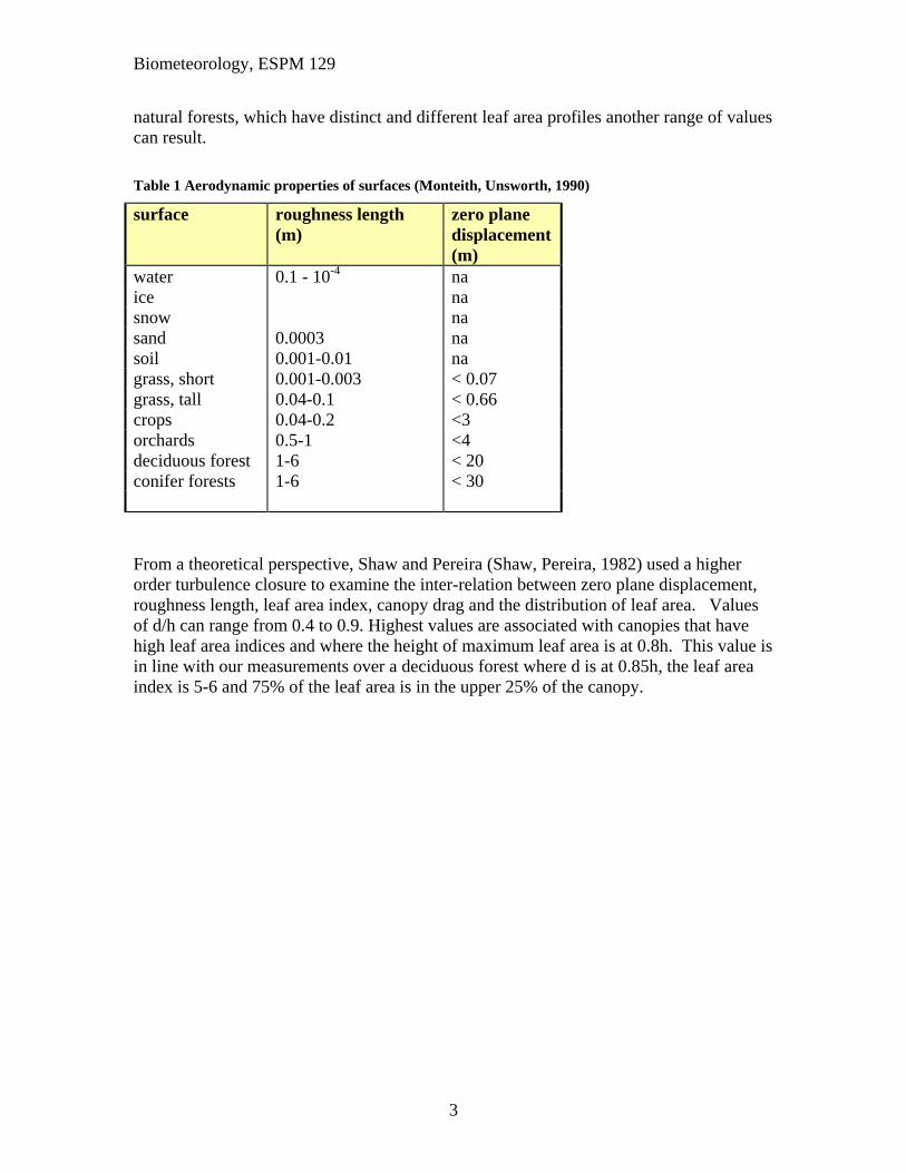
natural forests, which have distinct and different leaf area profiles another range of values can result.

Table 1 Aerodynamic properties of surfaces (Monteith, Unsworth, 1990)

surface roughness length (m)

zero plane displacement(m)

water 0.1 - 10-4 na ice na snow na sand 0.0003 na soil 0.001-0.01 na grass, short 0.001-0.003 < 0.07 grass, tall 0.04-0.1 < 0.66 crops 0.04-0.2 <3 orchards 0.5-1 <4 deciduous forest 1-6 < 20 conifer forests 1-6 < 30 From a theoretical perspective, Shaw and Pereira (Shaw, Pereira, 1982) used a higher order turbulence closure to examine the inter-relation between zero plane displacement, roughness length, leaf area index, canopy drag and the distribution of leaf area. Values of d/h can range from 0.4 to 0.9. Highest values are associated with canopies that have high leaf area indices and where the height of maximum leaf area is at 0.8h. This value is in line with our measurements over a deciduous forest where d is at 0.85h, the leaf area index is 5-6 and 75% of the leaf area is in the upper 25% of the canopy.


4

Figure 2 Computations of normalized zo as a function of leaf area distribution and leaf area index (Shaw, Pereira, 1982)


5

Figure 3 (Shaw, Pereira, 1982)

Raupach (Raupach, 1994) developed analytical equations for expressing zo and d as a function of leaf area index and canopy height. This enables one to construct general functions of zo and d without going to the detail of the work of Shaw and Pereira. Raupach reports that functions to be used include:

11

d

h

aL

aL

exp( )

a is a free variable, 7.5

z

h

d

hk u uo

h h ( )exp( / )*1

He assumes that u(h)/u* is about 3.3 for canopies with leaf areas greater than about 1, a reasonable assumption, as we will see later.


6

Figure 4 Computations of normalized d and zo as a function of leaf area index

Tall vs short Vegetation and Wind Profiles What happens when one removes vegetation from a landscape? Obviously the direct effects are a reduction in zero plane displacement and roughness length. But we also see a change in friction velocity, because the canopy drag coefficient and wind shear are reduced too when one removes a forest vegetation

u C ud*2 2

u kzu

z* ~

Leaf Area Index

0.1 1 10

d/h

or

z o/h

0.0

0.2

0.4

0.6

0.8

1.0theory of Raupach (1994)

d/h

zo/d


7

u

z

10

10

u

z

10

15

u kzu

z* ~

Let’s assume the forest is 30 m tall, its d is 18 m, and its z0 is 3 m. Let’s also assume the grass is 0.5 m, its d is 0.3 m and its z0 is 0.05 m what happens at z = 40?

u z

u z

u

u

z d

z

z d

z

u

ugrass

forest

grass

forest

grass

grass

forest

forest

grass

forest

( )

( )ln( ) / ln( ) .*

*, | |

*

*,

L

NMMOQPP

0 0

339

u z

u z

u

u

u

ugrass

forest

grass

forest

grass

forest

( )

( )ln(

.

.) / ln( ) .*

*,

*

*,

L

NMOQP

40 0 3

0 05

40 18

3339

If we assume that u is the same initially over the two sites at some elevated reference height, like 40 m, then we can solve for the ratios of friction velocity.


8

u

uforest

grass

*,

*

. 339

For the situation of our work in California, where we are studying an oak woodland and a short grassland we see that u* differs by more than a factor of 2.54 on an annual basis (0.149 vs 0.379 m s-1, grass and oak forest respectively).

u*, oak woodland, daily average

0.0 0.2 0.4 0.6 0.8 1.0

u*,

gras

slan

d, d

aily

ave

rage

0.0

0.1

0.2

0.3

0.4

0.5

2002

Secondary effects will be attributed to changes in thermal stratification, as we change the surface Bowen ratio and energy partitioning, which we discuss in the next section L18.2 Wind Profiles and Thermal Stratification The behavior of wind profiles differs dramatically under convective buoyant and stable conditions, which suppress turbulence. If one is at a reference height some distance above a crop or forest, wind speeds will be greater at the canopy interface under convective conditions than during stable night-time conditions. Evidence comes from everyday experience when one feels a diminishment of wind after sunset. If on uses the top of the canopy as a reference point then one experiences less wind with height than under stable conditions.


9

Figure 5 Wind profiles under different thermal stratification cases. Friction velocity was 0.3 m s-1 fore each case.

We can also examine the wind profile relative to a reference wind velocity

Wind Velocity

0 1 2 3 4 5 6

heig

ht (

m)

0

1

2

3

4

5

6

unstablenear neutralstable


10

Wind Velocity

0 1 2 3 4 5 6 7 8 9 10

heig

ht (

m)

0

1

2

3

4

5

6

stablenear neutralunstable

Figure 6 computations of wind speed profiles for unstable (z/L=-1), near neutral (z/L=0) and stable (z/L=0.2) thermal stratification. Friction velocity is 0.3 m s-1.

The key point is that shear increases under stable stratification so the momentum transfer at the surface can balance the momentum input from aloft. Note the results in Figure 4 are more realistic as one will not achieve wind speeds of 5 m s-1 under stable conditions and a u* of 0.3. Experimental data supports the theoretical calculations


11

Figure 7Data showing wind profiles over jack pine under different thermal stratification cases

Conceptually, the momentum of the free air in the surface boundary layer must find a sink at the ground. At night as stable thermal stratification intensifies, wind shear must increase in order to compensate for reduced turbulent mixing under stable conditions. In extreme conditions, elevated jets are observed a few tens of meters above the surface, where the local wind velocity may be relatively calm. The Monin-Obukhov Similarity Theory allows us to predict the behavior of wind profiles under stable and unstable conditions (Hogstrom, 1996; Wyngaard, 1992). A non-dimensional wind velocity gradient can be defined as a function of a non-dimensional height, z/L:

m

z

L

kz

u

u

z( )

*

L is the Monin-Obukhov length scale. It is defined using the turbulent kinetic energy budget or by using scaling arguments (eg Buckingham Pi theory).

U/Uref

0.6 0.7 0.8 0.9 1.0 1.1

z-d

(m

)

10

11

12

13

14

15

16

17

daytime, well mixed

night, stable stratification

Boreal Forestdata of Chris Vogel


12

From a physical view point, z/L is the ratio between of the buoyant production of

turbulent kinetic energy, gw v

v

' '

, to the shear production ( w uu

z' '

).

Remember a simple expression of the tke budget is:

w uu

z

gw

vv' ' '

normalizing by the shear term we arrive at:

1 3 z L kz u/ / * Under neutral conditions, z/L equals zero, so

kz

u

*3

1

Or the dissipation rate, , equals

u

kz*3

As a side note, for tall vegetation we define

u

z

u

k z d

z d

Lm*

( )(

( ))

One can also define a dimensionless temperature gradient

h

kz

z

*

For the surface layer

*

'

*

'w

uv


13

Monin-Obukhov theory says little about the behavior of z/L. This must be obtained from empirical evidence. It does, however, give us a framework for synthesizing field data. The ‘phi’ function has 3 asymptotic limits. 1. Under neutral conditions z/L approaches zero and phi approaches 1. 2. Under unstable conditions z/L approaches negative infinity. At the extreme case wind speeds are very light and free convection occurs. In this situation friction velocity is not the appropriate scaling velocity. Instead, a convective scaling velocity (w*) relevant

w z g wi v v*'

/

( ( / ) ' ) 1 3

3. Under stable conditions, dimensionless groups are independent of height. There is a decoupling between turbulent flow at various layers. Local wind shears and heat fluxes are important rather than surface layer turbulence. This conditions is called z-less stratification.

We stress at this point that M-O theory is valid for the surface boundary layer, not the mixed or planetary boundary layer.

Empirical algorithms for phi is

( / ) ( / )z L z L 1 And its functional response curve is noted in the following.


14

Figure 8 Non-dimensional wind shear coefficient for momentum

Typical model coefficients from field studies are listed below for unstable and stable conditions.

z/L

-12 -10 -8 -6 -4 -2 0 2

m

0

1

2

3


15

Figure 9 Survey by Hogstrom(Hogstrom, 1996)


16

Figure 10 Hogstrom 1988

Table 2 Parameters for Phi functions for momentum transfer, unstable thermal stratification

Citation k Businger (1971) 0.35 -15 -1/4 Dyer (1974) 0.41 -16 -1/4 Dyer and Bradley (1982) 0.40 -28 -1/4 Hogstrom (1988, 1996) .40 -19.3 -1/4

Table 3 Parameters for Phi functions for momentum transfer, stable thermal stratification

Citation k Businger (1971) 0.35 4.7 1 Dyer (1974) 0.41 5 1 Dyer and Bradley (1982) Hogstrom (1988, 1996) 0.40 5.3 1


17

Table 4 Parameters for Phi functions for heat transfer, unstable thermal stratification

Citation K Businger (1971) 0.35 -9 -1/2 Dyer (1974) 0.41 -16 -1/2 Dyer and Bradley (1982) 0.40 -14 -1/2 Hogstrom (1988) 0.40 -11 -1/2

Table 5 Parameters for Phi functions for heat transfer, stable thermal stratification

Citation k Businger (1971) 0.35 4.7 1 Dyer (1974) 0.41 5 1 Dyer and Bradley (1982) Hogstrom (1988) 0.40 7.8 1 Businger et al

m

z

L

kz

u

U

z

z

L( ) ( . )

*

1 4 7

Businger et al.

H

z

L

kz

z

z

L( ) . .

*

0 74 4 7

Dyer (1974)

H

z

L

kz

z

z

L( )

*

1 5

Near Neutral Boundary Layer

m

z

L

kz

u

U

z( )

*

1


18

H

z

L

kz

z( ) .

*

0 74

Convective or unstable boundary Layer

m

z

L

kz

u

U

z

z

L( ) ( )

*

/

1 15 1 4

Businger et al, using k=0.35 found

H

z

L

kz

z

z

L( ) . ( )

*

/

0 74 1 9 1 2

Dyer (1974) using k=0.41 found

H

z

L

kz

z

z

L( ) ( )

*

/

1 16 1 2


19

Figure 11 survey by Hogstrom (1996)

We can extend this theory and derive an integrated form of the wind profile that is corrected for stability effects.

u zu

k

z d

z

z d

L

z

Lm m( ) (ln( ) ( ) ( )*

0

0

normally zo <<<L, so the last term is close to zero. Stable Conditions

( ) 4.7m

z z

L L

Unstable Conditions

2

2 11 1( ) ln[( ) ( )] 2 tan ( )

2 2 2

z x xx

L

where


20

xz

L ( ) /1 15 1 4

Because there were issues with regards to the choice of the von Karman constant during the pioneering field studies, there have been subsequent updating of MO equations (Foken, 2006; Hogstrom, 1996). As a closing word of caution, M-O theory suffers from autocorrelation, where independent and dependent variables are inter-related (see Hicks, 1981, BLM 21,389; Mahrt, 1999, BLM.). Hence, many investigators prefer to use an independent measure of thermal stratification. Another measure of thermal instability is the Richardson number: Richardson Number

Ri

gz

uz

v

v

( )2

Flux Richardson

Rkzgw

w u u zf

v

v

' '

' '

for near neutral conditions Rf and z/L are equal. Gradient Richardson number

RK

KRif

m

H

18.3 Eddy Exchange Coefficients, Influence of Scalar, Stability and Roughness Sublayer With regard to M-O theory several layers of importance exist (Mahrt, 1999). So far we have discussed the surface layer where fluxes are constant with height and the flux gradient relation is a function of z/L. Above the surface layer, fluxes are not height independent and M-O theory fails.. However, local fluxes and scaling can be used with


21

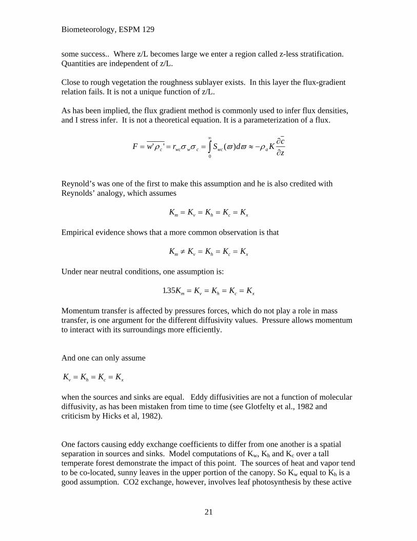
some success.. Where z/L becomes large we enter a region called z-less stratification. Quantities are independent of z/L. Close to rough vegetation the roughness sublayer exists. In this layer the flux-gradient relation fails. It is not a unique function of z/L. As has been implied, the flux gradient method is commonly used to infer flux densities, and I stress infer. It is not a theoretical equation. It is a parameterization of a flux.

F w r S d Kc

zc wc w c wc a

z' ' ( ) 0

Reynold’s was one of the first to make this assumption and he is also credited with Reynolds’ analogy, which assumes

K K K K Km v h c x Empirical evidence shows that a more common observation is that

K K K K Km v h c x Under near neutral conditions, one assumption is:

135. K K K K Km v h c x Momentum transfer is affected by pressures forces, which do not play a role in mass transfer, is one argument for the different diffusivity values. Pressure allows momentum to interact with its surroundings more efficiently. And one can only assume K K K Kv h c x when the sources and sinks are equal. Eddy diffusivities are not a function of molecular diffusivity, as has been mistaken from time to time (see Glotfelty et al., 1982 and criticism by Hicks et al, 1982). One factors causing eddy exchange coefficients to differ from one another is a spatial separation in sources and sinks. Model computations of Kw, Kh and Kc over a tall temperate forest demonstrate the impact of this point. The sources of heat and vapor tend to be co-located, sunny leaves in the upper portion of the canopy. So Kw equal to Kh is a good assumption. CO2 exchange, however, involves leaf photosynthesis by these active


22

leaves and soil respiration, about 20 m away. In this case Kc does not equal Kw and is smaller by 10 to 20 %. Differential source-sink locations and processes are a reason why Km does not equal the scalar values. Investigators have developed algorithms, that are stability dependent, to correct these values for one another. K ku z d z Lm m *( ) / ( / ) K ku z d z Lh h *( ) / ( / ) Unstable K

K

K

KRih

m

w

m

( ) .1 0 25 (Dyer and Hicks, 1970)

K

K

K

Kz Lh

m

w

m

( | / |) .1 16 0 25

Stable K

K

K

Kh

m

w

m

1 (Webb, 1970)


23

Figure 12Computations of eddy exchange coefficients for water, heat and CO2 with a biophysical model (CANOAK) that uses Lagrangian diffusion theory.

Roughness Sublayer K theory is notorious for its failure in a zone called the roughness sublayer. It is a region in the internal surface boundary layer, immediately adjacent to the vegetation. The roughness sublayer can extend 2 to 3 canopy heights, as it is directly affected by the influence of local trees or plants. In this zone Monin-Obukhov similarity theory fails. Work in the roughness sublayer has been limited because of weak gradients in well mixed turbulence and the need for access to tall towers. Investigators commonly examine the roughness enhancement factor. It is the ratio of the observed K to that computed from Monin-Obukhov scale theory

e

obs

mo

mo

obs

K

K

z L

( / )

Classic and pioneering work by Raupach (Raupach, 1979) indicated that the enhancement factor was on the order of 2. Simpson et al, (Simpson et al., 1998) revisited the problem

Kw (m2 s-1)

0 2 4 6 8 10

Kx

(m2 s

-1)

0

2

4

6

8

10

KcKh


24

with modern instrumentation and were able to study the problem over the course of a growing season show a distinct effect of leaf area and thermal stratification. Table 6 Enhancement factors for Kco2, forest with leaves Simpson et al. 1998. height unstable Near neutral Stable 1.9-2.2h 0.92 1.18 1.18 1.6-1.9h 1.23 1.27 1.52 1.4-1.6h 1.64 1.31 1.49 1.2-1.4h 1.60 1.57 1.66 Table 7 Simpson et al. 1998 enhancement factors for K co2, Forest with senescent leaves height unstable Near neutral Stable 1.9-2.2h 0.90 1.38 1.27 1.6-1.9h 0.84 1.52 1.49 1.4-1.6h 0.93 1.35 1.47 1.2-1.4h 1.20 1.88 1.92 They conclude that the roughness sublayer extended to about 2 times canopy height. We can use the conservation equation for a scalar flux covariance, w c' ' , to arrive at a theoretical understanding why K theory fails in the roughness sublayer.

w c

tw

c

z

w w c

zc

p

zg

c' ''

' ' ''

' ' '0 2

The steady state balance in a scalar covariance budget is a function of shear production, turbulent transport, pressure production and buoyancy production. A common parameterization of the pressure term is as a function of the flux covariance and a time scale:

cp

z

w c'

' ' '

On re-substitution (and assuming near neutral thermal stratification) we have a new equation for the flux covariance:


25

w cw c

z

w w c

z' '

' ' ' '

2

The first term on the RHS is equivalent to K dc/dz. The second term is a transport term. In essence, conventional flux gradient theory fails when the turbulent transport term is non-zero. Our data shows this to be true in the layer up to about 1.5h. High above vegetation canopies the turbulent transport term is nill (Meyers and Paw U, 1986). As a closing note, I want to stress that one should never attempt to apply Flux-Gradient theory by placing one instrument in the canopy and another above it. I have seen this done by colleagues with faint acquaintance of micrometeorology and it is a violation of the concepts discussed so far. K theory is not valid in the mixed layer either. 18.4 Wind Flow over hills. Natural landscape often are often not flat. Looking out the window of an aircraft flying across the United States one will observe foothills, mountain ranges, isolated hills, deep valleys, and plateaus, among other geographic features. Landscape features have distinct climates and meteorology. Their physical presence forces them to be immersed into different regions of the atmosphere, which have different temperatures (due to adiabatic cooling or heating) and different wind speeds. The physical upward or downward motion, know in the front or lee of hills causes orographic clouds to form, altering precipitation. Hills, mountains and valleys perturb air movement. With the presence of hills, wind flow must flow over and around them, causing flow to accerlerate, decelerate and separate. Mountain ranges and valleys channel flow and systematic heating and cooling of hills causes preferential flow up and down them. In this section we will overview how wind, turbulence and trace gas fluxes are affected by hills and slopes. Theoretically, the momentum budget, for two dimensional wind flow over a hill can be expressed in terms of a balance between advection, pressure gradients and shear stress gradients (Finnigan, Whiteman; Raupach and Finnigan, 1998; Belcher and Hunt (1998) ):

uu

zw

u

x

p

x z

A summary of how wind is perturbed by a hill is catalogued below. Winds: neutral thermal stratification


26

a. Maximum wind speed is near the crest b. Minimum wind speed is in the valley c. In the lee of the hill flow separation and reversed flow may occur

Winds: stable thermal stratification

d. flow over the crest of the hill can generate waves. e. Streamlines rise and decelerate upwind f. Streamlines descend and accelerate on lee side g. Point of maximum wind speed is on the lee side of the hill h. Gravity waves extract energy and momentum from mean flow i. Strong stable stratification may block flow over the hill and force

it around the hill

Thermally forced topographic flows a. temperature differences force upslope (anabatic) and downslope

(katabatic) winds Hills and mountains affect biometeorological processes in other ways, besides perturbing wind fields. Slope and azimuth of the landscape also affects the weathering and generation of soils (Jenny, 1980), soil moisture, plant types, height, leaf area index, available energy, and surface conductance (Raupach and Finnigan, 1996; Figure 9). During a trip to Innsbruck in the Austrian Alps, I noticed that Scots pine (Pinus sylvestris) existed on xeric, drier mountain faces, as they are better adapted to dry sites and support a relatively low leaf area index. On the wetter and more favorable faces existed denser stands of Norway spruce (Picea abies). As one walked up the mountain, another transition took place, Picea abies were slowly replaced with Pinus cembra, a low laying pine, almost shrub like. High elevations experience lower air temperatures. There is also a disturbance factor with the highest elevations and steepest mountains. Avalanches are very common and effectively remove vegetation, catastrophically.


27

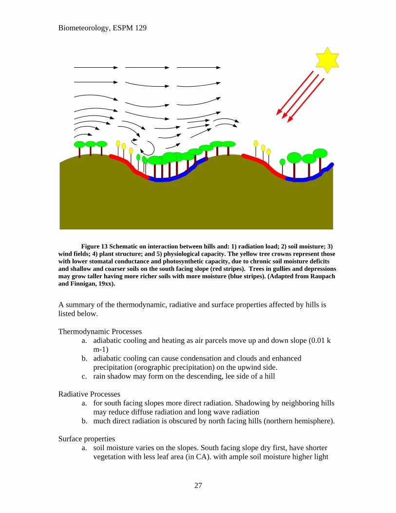
Figure 13 Schematic on interaction between hills and: 1) radiation load; 2) soil moisture; 3) wind fields; 4) plant structure; and 5) physiological capacity. The yellow tree crowns represent those with lower stomatal conductance and photosynthetic capacity, due to chronic soil moisture deficits and shallow and coarser soils on the south facing slope (red stripes). Trees in gullies and depressions may grow taller having more richer soils with more moisture (blue stripes). (Adapted from Raupach and Finnigan, 19xx).

A summary of the thermodynamic, radiative and surface properties affected by hills is listed below. Thermodynamic Processes

a. adiabatic cooling and heating as air parcels move up and down slope (0.01 k m-1)

b. adiabatic cooling can cause condensation and clouds and enhanced precipitation (orographic precipitation) on the upwind side.

c. rain shadow may form on the descending, lee side of a hill Radiative Processes

a. for south facing slopes more direct radiation. Shadowing by neighboring hills may reduce diffuse radiation and long wave radiation

b. much direct radiation is obscured by north facing hills (northern hemisphere). Surface properties

a. soil moisture varies on the slopes. South facing slope dry first, have shorter vegetation with less leaf area (in CA). with ample soil moisture higher light


28

may force a higher surface conductance. As soils dry, surface conductance diminishes

b. North facing has a more favorable soil water balance, denser vegetation. c. Position relative to orographic precipitation and prevailing winds may offset

some of the slope radiative losses. d. Soil moisture will be higher in the valleys and gulleys as rain water runoff

drains. We see in the grasslands of CA that oak belts will form in gulleys, as lateral flow enhances the amount of water available at preferred sites. The gulley is effectively able to mine rain from a larger area and enhance its climatological input.

Soil Texture (Jenny) Summary Points

Over tall vegetation the logarithmic wind profile is adjusted by incorporation of the zero plane displacement, d.

u zu

k

z d

z( ) ln( )*

0

The zero plane displacement represents the ‘center of pressure’ or the mean height of momentum absorption by a tall canopy. As a rule of thumb it is about 60% of canopy height, but will very with leaf area index and the vertical profile of leaf area index.

The roughness length is about 10% of canopy height Momentum transfer is greater over tall rough vegetation than short smooth

vegetation, given the same wind speeds aloft. Stable and unstable thermal stratification will alter the wind gradient relationship

u

z

u

k z d

z d

Lm*

( )(

( ))

A non-dimensional shear function has been defined empirically and is a function of the Monin Obuhukov scale length.

m

z

L

kz

u

u

z( )

*

The non-dimensional Monin-Obhukov length scale is defined as the ratio between buoyant and shear production of turbulent kinetic energy. It can also be defined with non-dimensional analysis using Buckingham pi theory.

z

L

kzgw

u

gw w u

u

zv

v vv

'{ ' } / { ' ' }

*

3

Non-dimensional wind shear is greater than one when thermal statification is stable; wind shear must increase to transfer momentum to the surface. Non-dimensional wind shear is less than one when thermal stratification is unstable. Non-dimensional wind shear equalsone when thermal stratification is neutral.


29

Eddy exchange coefficients are enhanced in the roughness sublayer (~1 to 1.5 h) due to large scale transport of momentum. Monin-Obuhkov scaling theory fails in this region.

Reynolds analogy assumes the eddy exchange coefficients for heat, water and momentum are equal. This assumes that the sources and sinks for these quantities are identical. In practice this is not true as momentum transfer is affected by pressure fluctuations and the other scalars are not. Plus CO2 exchange may have distributed sources and sinks in the vegetation and soil.

References: Arya, S. P. 1988. Introduction to Micrometeorology. Academic Press. Blackadar, A.K. 197. Turbulence and Diffusion in the Atmosphere, Springer Finnigan J (2000) Turbulence in Plant Canopies. Annu. Rev. Fluid Mech. 32, 519-571. Garratt, J.R. 1992. The Atmospheric Boundary Layer. Cambridge Univ Press. 316 pp. Kaimal, J.C. and J.J. Finnigan. 1994. Atmospheric Boundary Layer Flows: Their Structure and Measurement. Oxford Press. Panofsky, H.A. and J.A. Dutton. 1984. Atmospheric Turbulence. Wiley and Sons, 397 pp. Raupach, M.R., R.A. Antonia and S. Rajagopalan. 1991. Rough wall turbulent boundary

layers. Applied Mechanics Reviews. 44, 1-25. Raupach, MR and Finnigan, JJ. 1997. The influence of topography on meteorological variables and surface-atmosphere interactions. 190, 182-213 Shaw, R. 1995. Lecture Notes, Advanced Short Course on Biometeorology and

Micrometeorology. Stull, R.B. 1988. Introduction to Boundary Layer Meteorology. Reidel Publishing.

Dordrect, The Netherlands. Thom, A (1975). Momentum, Mass and Heat Exchange of Plant Communities. In;

Vegetation and the Atmosphere, vol 1. JL Monteith, ed. Academic Press. EndNote References


30

Foken T (2006) 50 years of the Monin-Obukhov similarity theory. Boundary-Layer

Meteorology 119, 431-447. Hogstrom U (1996) Review of some basic characteristics of the atmospheric surface

layer. Boundary-Layer Meteorology 78, 215-246. Monteith JL, Unsworth MH (1990) Principles of Environmental Physics Edward Arnold,

London. Raupach MR (1979) Anomalies in Flux-Gradient Relationships over Forest. Boundary-

Layer Meteorology 16, 467-486. Raupach MR (1994) Simplified expressions for vegetation roughness length and zero-

plane displacement as functions of canopy height and area index. Boundary Layer Meteorology 71, 211-216.

Raupach MR, Thom AS (1981) Turbulence in and above Plant Canopies. Annual Review of Fluid Mechanics 13, 97-129.

Shaw RH, Pereira AR (1982) Aerodynamic roughness of a plant canopy: A numerical experiment. Agricultural Meteorology 26, 51-65.

Simpson IJ, Thurtell GW, Neumann HH, Den Hartog G, Edwards GC (1998) The validity of similarity theory in the roughness sublayer above forests. Boundary-Layer Meteorology 87, 69-99.

Wyngaard JC (1992) Atmospheric-Turbulence. Annual Review of Fluid Mechanics 24, 205-233.

Lecture 18 Wind and Turbulence Part 3 Surface Boundary … · Biometeorology, ESPM 129 2 Thom...

Documents

Transcript of Lecture 18 Wind and Turbulence Part 3 Surface Boundary … · Biometeorology, ESPM 129 2 Thom...