Lecture 18: Prediction in Survival

Predicted survival probabilityC-indices and other performance measures

Predicting Survival Probability

• There are two potential goals in modeling time to event data– Test a hypothesis about associations between a

covariate and survival controlling for other factors– Predictive modeling

• It is often of interest to predict survival probability for a new patient given their specific covariates

Predicting Survival Probability

• Cox regression returns coefficients estimates but how do we make a prediction?

• Let t1 < t2 < … < tD be distinct event times and di = indicator of event at time ti

• We can estimate a cumulative hazard by:

1

0 ;

; exp

ˆi

i

ii

p

i h jhj R t h

d

W tt t

W t b Z

H t

b

b

Predicting Survival Probability

• From this we obtain the estimate of the baseline survival probability

• The estimated survival probability for a subject with covariate vector Z0 is:

0 0 ;ˆ ˆexp exp i

ii

d

W tt tS t H t

b

'0exp

0 0ˆ ˆS t S t b zZ Z

Predicting Survival Probability

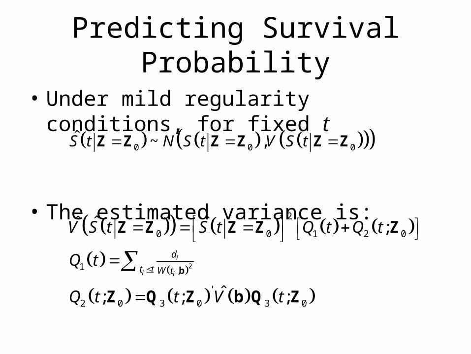
• Under mild regularity conditions, for fixed t

• The estimated variance is:

0 0 0ˆ ~ ,S t N S t V S t Z Z Z Z Z Z

2

2

0 0 1 2 0

1 ,

'

2 0 3 0 3 0

ˆ ˆˆ ;

ˆ; ; ;

i

i i

d

t t W t

V S t S t Q t Q t

Q t

Q t t V t

b

Z Z Z Z Z

Z Q Z b Q Z

Predicting Survival Probability

• Q3 is a vector of length p with kth element:

• Use estimated variance to construct CIs for the point estimate

3 0 0

'

;; , 1, 2,...,

; ;

; exp

i

i

ki i

kkt t i i

ki jk j

j R t

W t dQ t Z k p

W t W t

W t Z

bZ

b b

b bZ

Small Example

• Study examining exposure to hexachlorobenzene on survival in pancreatic cancer.

• 8 mice tansfected with pancreatic cancer cells and split into 2 groups:– Control animals – HBC exposed animals.

• Followed forward in time with a primary outcome of time to death.

Data and Cox Model

• Treatmen 0 = controls• Treatment 1 = HBC

exposed• Cox Model

Time Death Treatment Group

16 1 0

24 0 0

25 1 0

31 1 0

25 0 1

25 1 1

32 0 1

40 1 1

0 1

ˆ

exp 1.648*

ˆ 1.648

ˆ 1.356

treatmenth t Z h t I

Baseline Cumulative Hazard and Survival

ti di R(ti) 1ˆ ˆ; exp *

ii Trtj R t

W t I

ˆ;i id W t 0 ˆ;ˆ i

i i

d

t t W tH t

0 0

ˆ ˆexpS t H t

Estimated Survival Probabilities

• What is the survival probability that a mouse in group 0 survives to 25 weeks?

• What about a mouse in group 1?

• What is the survival probability that a mouse in group 0 survives to 35 weeks?

• What about a mouse in group 1?

R Examplelibrary(rms)Library(KMsurv)###BMT exampledata(bmt)colnames(bmt)<-c("dgroup","TTD","DFS","dead","relapse","Either","tAGVHD","AGvHD","tCGVHD", "CGvHD","tPR","PR","PtAge","DonAge","PtSex","DonSex","PtCMV","DonCVM","TTTrans", "FAB", "Hosp","MTX")bmt1<-bmt[sample(1:137, 137, replace=F),]bmt2<-bmt1[1:133,]st2<-Surv(bmt2$DFS, bmt2$Either)fit<-cph(st2 ~ factor(dgroup) + FAB + PtAge + DonAge + PtAge*DonAge, data=bmt2, x=TRUE, y=TRUE)

#Predicted survival probability at 6,12, 24 months and 1000 days#Note these predictions are for observations 135-137 which weren't used to build the modeltest<-bmt1[134:137,c(1,13,14,19,20)]survest(fit, test, times=c(182,365,730,1000), conf.type="log-log")

Test Data> fitcph(formula = st2 ~ factor(dgroup) + FAB + PtAge + DonAge + PtAge * DonAge, data = bmt2, x = T, y = T, surv = T)

Coef S.E. Wald Z Pr(>|Z|)dgroup=2 -0.9821 0.3578 -2.74 0.0061 dgroup=3 -0.2687 0.3745 -0.72 0.4731 FAB 0.7460 0.2829 2.64 0.0084 PtAge -0.0808 0.0361 -2.24 0.0252 DonAge -0.0809 0.0302 -2.68 0.0075 PtAge*DonAge 0.0030 0.0010 3.17 0.0015

> test<-bmt1[134:137,c(1,13,14,19,20)]> test dgroup PtAge DonAge FAB PtAge*DonAge exp(b’Z)107 3 39 48 1 1872 -0.923120 1 40 37 0 1480 -1.785393 3 18 23 0 414 -2.341866 2 33 28 0 924 -3.1417

Results> round(survest(fit, test, times=c(182,365,730,1000), conf.type="log-log")$surv, 4) 182 365 730 1000107 0.3403 0.1764 0.0464 0.042820 0.6309 0.4765 0.2692 0.260393 0.7716 0.6587 0.4777 0.468666 0.8891 0.8276 0.7154 0.7092

> round(survest(fit, test, times=c(182,365,730,1000), conf.type="log-log")$lower, 4) 182 365 730 1000107 0.5685 0.3984 0.1974 0.189520 0.7830 0.6669 0.4846 0.475693 0.8801 0.8114 0.6875 0.680866 0.9380 0.8982 0.8205 0.8160

> round(survest(fit, test, times=c(182,365,730,1000), conf.type="log-log")$upper, 4) 182 365 730 1000107 0.1278 0.0380 0.0030 0.002620 0.4202 0.2575 0.0928 0.087493 0.5906 0.4343 0.2330 0.224566 0.8060 0.7165 0.5673 0.5597

Discrimination in Survival

• Discrimination:– Quantify the ability of a model to correctly classify

subjects into categories defined by the model

• Where have you used this before?– AUC of ROC curve provides measure of

discrimination– How is AUC calculated?

Simple Case

• Single continuous predictor with a binary outcome

• Examine sensitivity and specificity at each possible cut point

• Develop and ROC curve – Sensitivity vs. (1-specificity)

• Estimate AUC of the resulting curve

C-Index

• In case of logistic regression, same thing as AUC from an ROC curve

• Example: Assume Xi = indicator of death• Assume:– Yi = predicted probability of death for patients with Xi

= 1

– Vi = predicted probability of death for patients with Xi = 0

• Definition of C (AUC of ROC curve)

C-index: Important Link

• Hanley and McNeill (1982) showed an link between the Mann Whitney U statistic and the C-index

• Demonstrated that AUC can be estimated using MWU

C-Index

• Definition of C (of AUC of ROC curve)– C = P(Y > V) for continuous Y and V– C = P(Y > V) + 0.5P(Y = V) for discrete Y and V

• Interpretation– The C statistic is the probability that a subject

from the event group has a higher predicted probability of having an event relative to subjects in the non-event group

C-index: Important Link

• Recall how MWU works:– For each pair of subjects (i, j) where the first is from

the non-event group and the other is from the event group• Assign Wij = 1 if Yi > Vj

• Assign Wij = 0.5 if Yi = Vj

• Assign Wij = 0 if Yi < Vj

• C = U/(kn) where k is the number of events and n is the number of non-events

• Note: kn = total number of pairs

Why is This Difficult for Survival?

• Discrimination not as clear for survival• We have whether or not a subject

experienced an event• However, we also have when they

experienced the event• In survival, we expect our model to correctly

distinguish between those that have shorter vs. longer survival times

What Can We Compare?

• What is a reasonable analogy in survival analysis?• Compare survival times of each pair of individuals• For each pair:– Determine which subject had event first– Determine which was predicted to have event first

• Estimate linear predictor for each• Larger linear predictor is first predicted to fail

– Is the pair concordant or discordant?• Estimate fraction of concordant pairs

Does This Work?

• Assuming NO censoring, yes it does• However, not so simple with censoring– How to define the survival times of censored

individuals?– Don’t want to delete censored observations as

they provide information on survival time• We need to define “usable” and “unusable”

pairs

Usable vs. Non-usable Pairs

• Useable pairs:– Both event times observed– Event time for one subject < censoring time for

the other subject• Unusable pairs:– Both events are censored– Event time for one subject > censoring time for

other subject

C-Index for Survival Analysis

• C-Index: Proportion of usable pairs in which the predictions and outcomes are concordant

• Probability of concordant and discordant pairs

& OR &

& &

& OR &

& &

c i j i j i j i j

i j i j i j i j

d i j i j i j i j

i j i j i j i j

P X X Y Y X X Y Y

P X X Y Y P X X Y Y

P X X Y Y X X Y Y

P X X Y Y P X X Y Y

C-Index for Survival Analysis

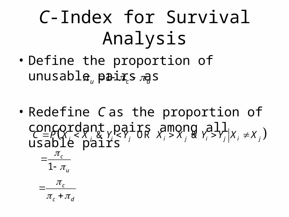
• Define the proportion of unusable pairs as

• Redefine C as the proportion of concordant pairs among all usable pairs

& OR &

1

i j i j i j i j i j

c

u

c

c d

C P X X Y Y X X Y Y X X

1u c d

Estimation

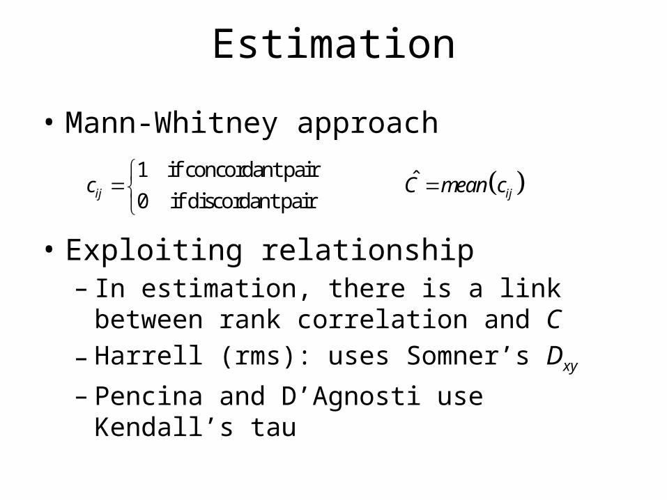
• Mann-Whitney approach

• Exploiting relationship– In estimation, there is a link between rank

correlation and C– Harrell (rms): uses Somner’s Dxy

– Pencina and D’Agnosti use Kendall’s tau

1 if concordant pair ˆ0 if discordant pairij ijc C mean c

Relationship Between tm and C

• Kendall’s tm is a non-parametric measure correlation between two variable defined as:

• The relationship between tm and C is

1c d c d

c d um

12 1

c

c d

m

C

Estimating tm and C

• The number of concordant and discordant pairs in the data are calculated according to:

• Use this information to estimate tm and C :

andh hj h hjh j h jc c d d

1 11 1

12

and

ˆˆ ˆ 1c d c

c d c d

c h d hN N N Nh h

p p pm mp p p p

p c p d

C

R Estimation

• “Hmisc” package– rcorr.cens function – Estimates multiple things (including Somner’s D

and C-index)

R Estimation> st<-Surv(bmt$DFS, bmt$Either)> fit<-cph(st~factor(dgroup)+TTTrans+FAB+PtAge+ DonAge+PtAge*DonAge, data=bmt, x=T, y=T, surv=T)> linpred<-fit$linear.predictors> cetal<-rcorr.cens(-linpred, st)> round(cetal, 4) C Index Dxy S.D. n missing 0.6671 0.3341 0.0651 137.0000 0.0000 uncensored Relevant Pairs Concordant Uncertain 83.0000 15540.0000 10366.0000 3078.0000

Alternatives of Prediction Performance

• There are MANY measures of prediction performance…

• Dxy: Somner’s D – rank correlation measure

• R2: Nagelkerke’s R2 – Generalized version of R2

• Slope: Calibration slope– Slope of line for predicted vs. observed

Alternatives of Prediction Performance

• D: Discrimination index– Model LR(c2 – 1)/n

• U: Unreliability index– Difference between -2LL for uncalibrated Xb and

Xb with slope/intercept calibrated for the test data

• Q: Overall quality index– D-U

Overly Optimistic

• The C-index based on the observed data is optimistic

• Why?– Applying same model to data that was used to

generate the model– Prediction measures will tend to be larger

• Better way– Apply model to new data– Use cross-validation or bootstrap approach

R Model Validation

> val<-validate(fit, B=250, dxy=TRUE)> round(val, 4) index.orig training test optimism index.corrected nDxy -0.3341 -0.3716 -0.3166 -0.0551 -0.2790 250R2 0.2167 0.2532 0.1835 0.0696 0.1471 250Slope 1.0000 1.0000 0.8284 0.1716 0.8284 250D 0.0433 0.0523 0.0358 0.0166 0.0267 250U -0.0027 -0.0027 0.0037 -0.0063 0.0037 250Q 0.0459 0.0550 0.0321 0.0229 0.0231 250

Note: in cph command, must include: x=T, y=T, surv=T

Corrected C = ½ (0.2790+1) = 0.6395 vs. 0.6671 originally

Why So Similar?

• Recall we had already done some model “validation” approaches – Model building used AIC

• Bootstrap approach to model building– Draw bootstrap sample– Find “best model” on bootstrap sample– Repeat N times– Final model: includes the covariates for which >50% of

samples included the covariate• Model was already “conservative” in including

covariates

Additional Info on C

• 95% confidence intervals helpful• Confidence intervals are usually reported with

AUC from an ROC• In R there is no function to estimate• Multiple methods for estimating CIs for the C-

index for a survival model have been posed

One Confidence Interval for C

• The CI based on C estimated using Kendall’s tau is:

2

4

ˆvar

2 24

11 2

11 2

11 2

ˆ

ˆwhere var 2

1

1

c d

P

N

d cc c d cd c ddp p

cc h hN N N h

dd h hN N N h

cd h hN N N h

C z

P p p p p p p p

p c c

p d d

p c d

CI in R> cetal<-rcorr.cens(-linpred, st)> round(cetal, 4) C Index Dxy S.D. n missing 0.6671 0.3341 0.0651 137 0.0000

uncensored Relevant Pairs Concordant Uncertain 83 15540 10366 3078

> c_hat_lo<-cetal[1]-1.96*cetal[3]/sqrt(cetal[4])> c_hat_lo 0.6561576

> c_hat_hi<-cetal[1]+1.96*cetal[3]/sqrt(cetal[4])> c_hat_hi 0.6779479

Multivariate Survival Analysis

• Up to this point, we have been assuming that event times between our i subjects are independent.

• In many survival studies this it true but…

• There are times when this assumption isn’t appropriate– Siblings/Families– Clustering

• School• Hospital

– Recurrent events • Hospitalization• Transplant rejection

Frailty Models

• Frailty model: an approach for modeling associations between the individual survival times within a subgroup

• Assumes there is an unobserved random effect (frailty) that acts multiplicatively on all members of a subgroup.

• Referred to as frailty because it is a measure of how much more or less likely the group is to experience the event relative to other groups.

Frailty Model

• So let’s look at the form of the frailty model

– i is the number of groups – j is the number of subjects in the ith group– h0(t) is still arbitrary baseline hazard rate

– Zij is the vector of covariates for the ijth subject

– wi are the frailties for each group

'0 exp , 1,2,..., ; 1,2,...,ij i ij ih t h t w i G j n Z

Comparing CPH and Frailty Models

• Recall our CPHM

• We can re-write our frailty model to look similar

'0 exp , 1,2,...,j jh t h t j n Z

Testing the Random Effect

• As previously mentioned, many survival data are independent…

• There are also times when it seems obvious that observations are correlated (e.g. siblings)

• But we can recall examples we’ve discussed so far where patients might be grouped

• Ideally we would like to be able to test whether or not we need a random effect

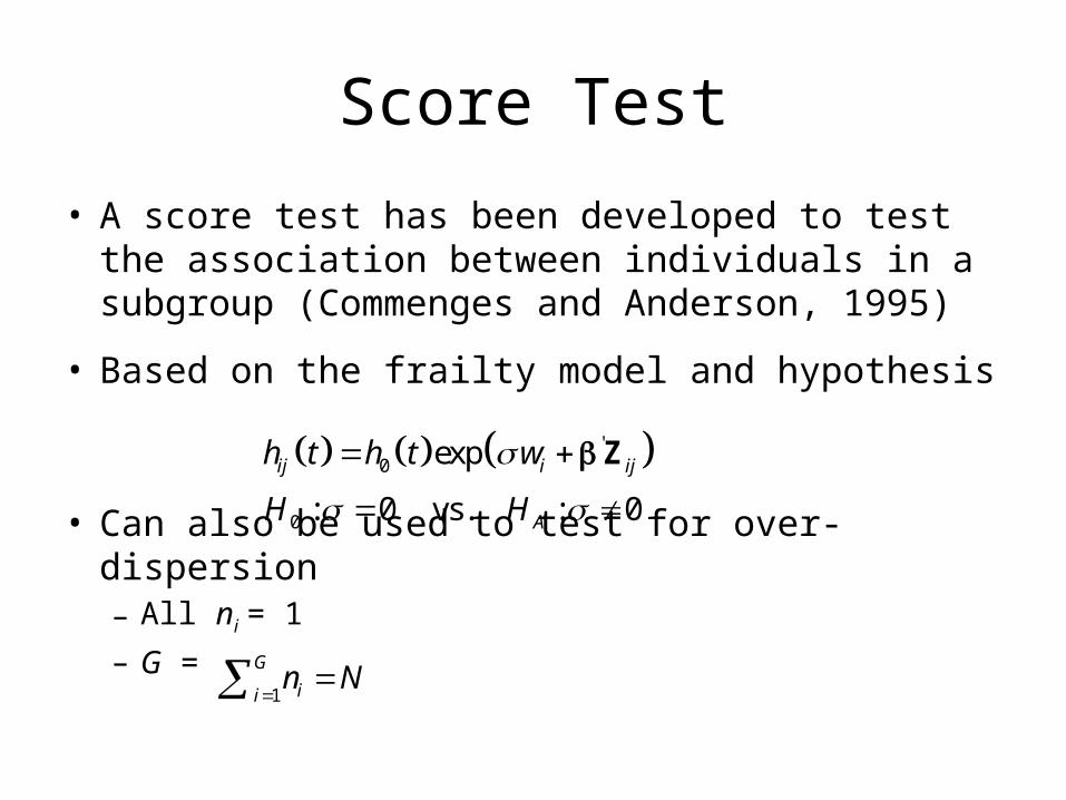
Score Test

• A score test has been developed to test the association between individuals in a subgroup (Commenges and Anderson, 1995)

• Based on the frailty model and hypothesis

• Can also be used to test for over-dispersion– All ni = 1

– G =

'0

0

exp

: 0 vs. : 0

ij i ij

A

h t h t w

H H

Z

1

G

iin N

Conducting the Score Test

• Fit a Cox PHM using event times Tij, dij, Zij.

• Using Yij(t) calculate:

• Calculate the Martingale residuals, Mij, from this model

'0 expij ijh t h tZ Z

0 '

1 1expiG n

ij iji jS t Y t

bZ

Conducting the Score Test

• The score statistic is given by.

• D is the total number of events• C is:

• Alternatively we can write the statistic as:

2

1 1

iG n

iji jT M D C

2

'21 1 1 10

expi iG n G nijhk ij hki j h k

ij

C Y TS T

bZ

211 1 1 1

i j iG n n G n

k ij ik iji j i jk j

T M M M N C

Conducting the Score Test

• The final test statistic is given by

• Where V is the estimated variance for the score statistic

• Under the null hypothesis, this statistic is asymptotically N(0,1)

T V

Uses of the Score Test

• Used to test for association of the random effect after adjusting for other covariates

• Test for over-dispersion in a Cox PH model

• Can also be applied in stratified Cox models

Estimation of The Model

• If we want to estimate a frailty model, we need to estimate:– Risk coefficients, b– Baseline hazard, h0(t)

– The frailty parameters, ui

• This means we need:– Likelihood– Algorithm for estimating the latent frailty terms, wi

Estimation of the Frailty Model

1. Assume some parametric form for ui

2. Assume either a semi-parametric or a parametric form for the triplet (Tij, dij, Zij)

3. Write out the log-likelihood4. If we assume a non-parametric form for h0(t),

then obtain using the EM algorithm.5. If we assume a parametric for, we can

maximize the likelihood directly

0ˆˆ ,H t

More About The Frailty Terms

• For estimation, we must assume some distribution for our frailty ui

• The most common shared frailty model assumes

• Thus the density function is:

1

1

1

1

u

u eg u

1 1,

1 &

iid

i

i i

u

E u Var u

Likelihood

• Likelihood still based on a covariate vector, Zij, observed times Tij, and an event indicator dij

• However, the likelihood also includes components to address the frailty component

1 11

'101

'01

, ln ln ln

ln 1 exp

ln

i

i

G

i ii

n

i ij ijj

n

ij ij ijj

l D D

D H T

h T

Z

Z

Shared Frailty Model in R

• We can use the frailtypack package in R to construct shared frailty models

• This package fits a penalized random effect likelihood– Penalizes the hazard function

• Reason for the penalized likelihood is that for small estimated of the frailty parameter, numeric problems may arise.

Example

• Evaluation of tumorigenesis in drug vs. placebo in rat model

• Study included 50 litter of rats – One rat/litter treated with drug– Two rats/litter treated with placebo

• Clearly rats from the same litter might be expected to be correlated

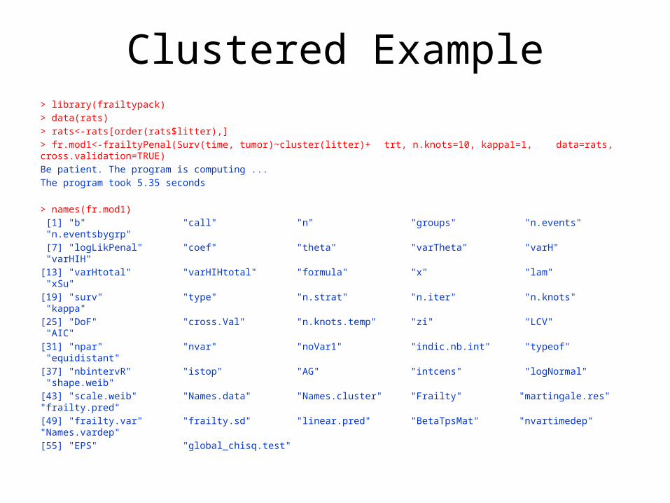
Clustered Example> library(frailtypack)> data(rats)> rats<-rats[order(rats$litter),]> fr.mod1<-frailtyPenal(Surv(time, tumor)~cluster(litter)+ trt, n.knots=10, kappa1=1, data=rats, cross.validation=TRUE)Be patient. The program is computing ... The program took 5.35 seconds

> names(fr.mod1) [1] "b" "call" "n" "groups" "n.events" "n.eventsbygrp" [7] "logLikPenal" "coef" "theta" "varTheta" "varH" "varHIH" [13] "varHtotal" "varHIHtotal" "formula" "x" "lam" "xSu" [19] "surv" "type" "n.strat" "n.iter" "n.knots" "kappa" [25] "DoF" "cross.Val" "n.knots.temp" "zi" "LCV" "AIC" [31] "npar" "nvar" "noVar1" "indic.nb.int" "typeof" "equidistant" [37] "nbintervR" "istop" "AG" "intcens" "logNormal" "shape.weib" [43] "scale.weib" "Names.data" "Names.cluster" "Frailty" "martingale.res" "frailty.pred" [49] "frailty.var" "frailty.sd" "linear.pred" "BetaTpsMat" "nvartimedep" "Names.vardep" [55] "EPS" "global_chisq.test"

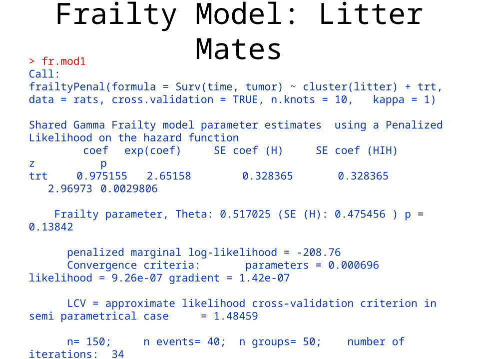
Frailty Model: Litter Mates> fr.mod1Call:frailtyPenal(formula = Surv(time, tumor) ~ cluster(litter) + trt, data = rats, cross.validation = TRUE, n.knots = 10, kappa = 1)

Shared Gamma Frailty model parameter estimates using a Penalized Likelihood on the hazard function coef exp(coef) SE coef (H) SE coef (HIH) z ptrt 0.975155 2.65158 0.328365 0.328365 2.96973 0.0029806

Frailty parameter, Theta: 0.517025 (SE (H): 0.475456 ) p = 0.13842 penalized marginal log-likelihood = -208.76 Convergence criteria: parameters = 0.000696 likelihood = 9.26e-07 gradient = 1.42e-07

LCV = approximate likelihood cross-validation criterion in semi parametrical case = 1.48459

n= 150; n events= 40; n groups= 50; number of iterations: 34 Exact number of knots used: 10 Best smoothing parameter estimated by an approximated Cross validation: 2.88636e-17, DoF: 9.00

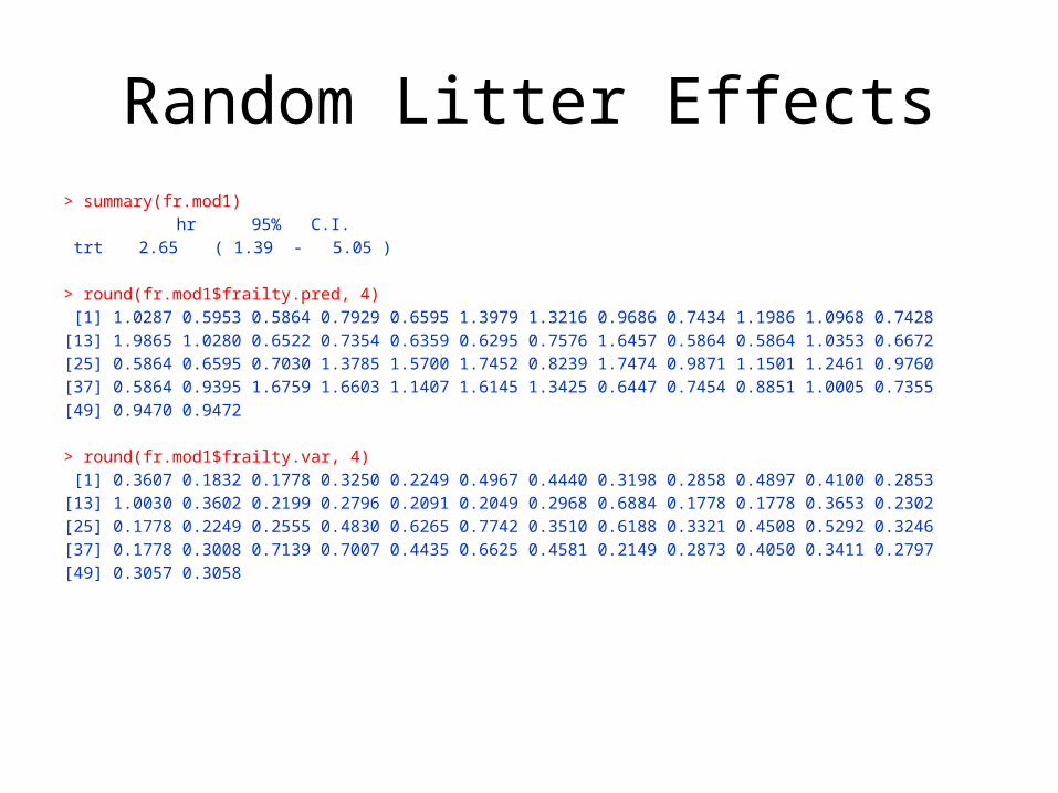
Random Litter Effects> summary(fr.mod1) hr 95% C.I. trt 2.65 ( 1.39 - 5.05 )

> round(fr.mod1$frailty.pred, 4) [1] 1.0287 0.5953 0.5864 0.7929 0.6595 1.3979 1.3216 0.9686 0.7434 1.1986 1.0968 0.7428[13] 1.9865 1.0280 0.6522 0.7354 0.6359 0.6295 0.7576 1.6457 0.5864 0.5864 1.0353 0.6672[25] 0.5864 0.6595 0.7030 1.3785 1.5700 1.7452 0.8239 1.7474 0.9871 1.1501 1.2461 0.9760[37] 0.5864 0.9395 1.6759 1.6603 1.1407 1.6145 1.3425 0.6447 0.7454 0.8851 1.0005 0.7355[49] 0.9470 0.9472

> round(fr.mod1$frailty.var, 4) [1] 0.3607 0.1832 0.1778 0.3250 0.2249 0.4967 0.4440 0.3198 0.2858 0.4897 0.4100 0.2853[13] 1.0030 0.3602 0.2199 0.2796 0.2091 0.2049 0.2968 0.6884 0.1778 0.1778 0.3653 0.2302[25] 0.1778 0.2249 0.2555 0.4830 0.6265 0.7742 0.3510 0.6188 0.3321 0.4508 0.5292 0.3246[37] 0.1778 0.3008 0.7139 0.7007 0.4435 0.6625 0.4581 0.2149 0.2873 0.4050 0.3411 0.2797[49] 0.3057 0.3058

Other Frailty Models

• We have focused on a shared frailty model – Include a single random effect– Can also be implemented for stratified Cox model

• There are alternative frailty models for more complex scenarios– Nested frailty model– Joint frailty model– Additive frailty model

More on frailtypack

• All 4 types of frailty model are implemented in this package– frailtyPenal function: Shared, nested and joint– additivePenal function: additive models

• The package includes examples with each function– More info: Rondeau et. al (2012). Frailtypack: An R package

for the analysis of correlated survival data… J Stat Software, 47(4).

• One draw-back is that we can not model interactions using the frailty functions in this package

Next Time

• Competing Risk Regression