Lecture 18: Elements of Dynamic Programming...
23
Lecture 18: Elements of Dynamic Programming COMS10007 - Algorithms Dr. Christian Konrad 02.04.2019 Dr. Christian Konrad Lecture 18: Elements of Dynamic Programming 1/ 8
Transcript of Lecture 18: Elements of Dynamic Programming...
Lecture 18: Elements of Dynamic ProgrammingCOMS10007 - Algorithms
Dr. Christian Konrad
02.04.2019
Dr. Christian Konrad Lecture 18: Elements of Dynamic Programming 1 / 8
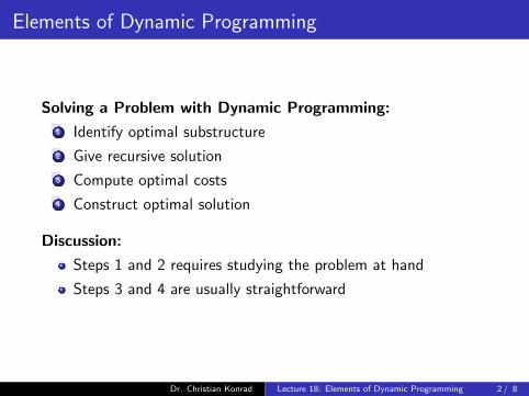
Elements of Dynamic Programming
Solving a Problem with Dynamic Programming:
1 Identify optimal substructure
2 Give recursive solution
3 Compute optimal costs
4 Construct optimal solution
Discussion:
Steps 1 and 2 requires studying the problem at hand
Steps 3 and 4 are usually straightforward
Dr. Christian Konrad Lecture 18: Elements of Dynamic Programming 2 / 8
Step 1: Identify Optimal Substructure
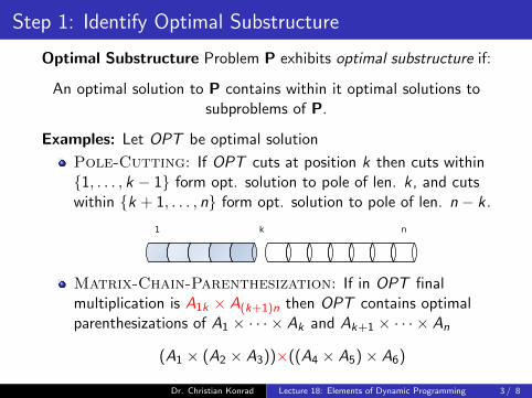
Optimal Substructure Problem P exhibits optimal substructure if:
An optimal solution to P contains within it optimal solutions tosubproblems of P.
Examples: Let OPT be optimal solution
Pole-Cutting: If OPT cuts at position k then cuts within{1, . . . , k − 1} form opt. solution to pole of len. k , and cutswithin {k + 1, . . . , n} form opt. solution to pole of len. n− k .
Matrix-Chain-Parenthesization: If in OPT finalmultiplication is A1k × A(k+1)n then OPT contains optimalparenthesizations of A1 × · · · × Ak and Ak+1 × · · · × An
(A1 × (A2 × A3))×((A4 × A5)× A6)
Dr. Christian Konrad Lecture 18: Elements of Dynamic Programming 3 / 8
Step 2. Give Recursive Solution
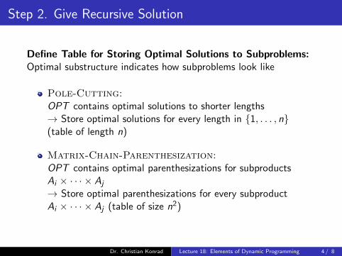
Define Table for Storing Optimal Solutions to Subproblems:Optimal substructure indicates how subproblems look like
Pole-Cutting:OPT contains optimal solutions to shorter lengths→ Store optimal solutions for every length in {1, . . . , n}(table of length n)
Matrix-Chain-Parenthesization:OPT contains optimal parenthesizations for subproductsAi × · · · × Aj
→ Store optimal parenthesizations for every subproductAi × · · · × Aj (table of size n2)
Dr. Christian Konrad Lecture 18: Elements of Dynamic Programming 4 / 8
Step 2. Give Recursive Solution (2)
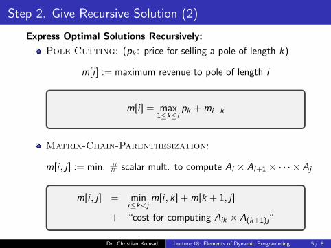
Express Optimal Solutions Recursively:
Pole-Cutting: (pk : price for selling a pole of length k)
m[i ] := maximum revenue to pole of length i
m[i ] = max1≤k≤i
pk + mi−k
Matrix-Chain-Parenthesization:
m[i , j ] := min. # scalar mult. to compute Ai × Ai+1 × · · · × Aj
m[i , j ] = mini≤k<j
m[i , k] + m[k + 1, j ]
+ “cost for computing Aik × A(k+1)j”
Dr. Christian Konrad Lecture 18: Elements of Dynamic Programming 5 / 8
Compute Optimal Costs
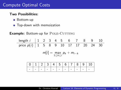
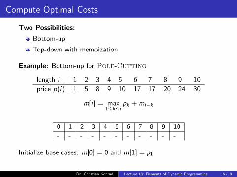
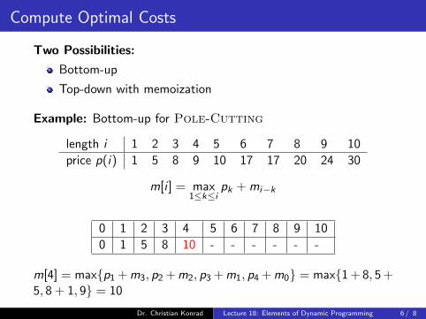
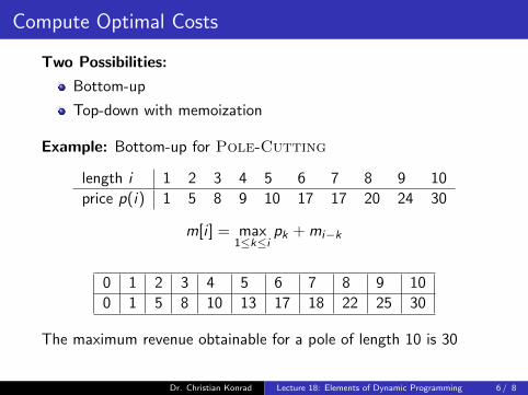
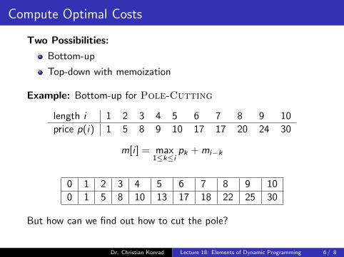
Two Possibilities:
Bottom-up
Top-down with memoization
Example: Bottom-up for Pole-Cutting
length i 1 2 3 4 5 6 7 8 9 10
price p(i) 1 5 8 9 10 17 17 20 24 30
m[i ] = max1≤k≤i
pk + mi−k
0 1 2 3 4 5 6 7 8 9 10
- - - - - - - - - - -
Dr. Christian Konrad Lecture 18: Elements of Dynamic Programming 6 / 8
Compute Optimal Costs
Two Possibilities:
Bottom-up
Top-down with memoization
Example: Bottom-up for Pole-Cutting
length i 1 2 3 4 5 6 7 8 9 10
price p(i) 1 5 8 9 10 17 17 20 24 30
m[i ] = max1≤k≤i
pk + mi−k
0 1 2 3 4 5 6 7 8 9 10
- - - - - - - - - - -
Initialize base cases: m[0] = 0 and m[1] = p1
Dr. Christian Konrad Lecture 18: Elements of Dynamic Programming 6 / 8

Compute Optimal Costs
Two Possibilities:
Bottom-up
Top-down with memoization
Example: Bottom-up for Pole-Cutting
length i 1 2 3 4 5 6 7 8 9 10
price p(i) 1 5 8 9 10 17 17 20 24 30
m[i ] = max1≤k≤i
pk + mi−k
0 1 2 3 4 5 6 7 8 9 10
0 1 - - - - - - - - -
m[2] = max{p1 + m1, p2 + m0} = max{1 + 1, 5 + 0} = 5
Dr. Christian Konrad Lecture 18: Elements of Dynamic Programming 6 / 8
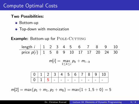
Compute Optimal Costs
Two Possibilities:
Bottom-up
Top-down with memoization
Example: Bottom-up for Pole-Cutting
length i 1 2 3 4 5 6 7 8 9 10
price p(i) 1 5 8 9 10 17 17 20 24 30
m[i ] = max1≤k≤i
pk + mi−k
0 1 2 3 4 5 6 7 8 9 10
0 1 5 - - - - - - - -
m[2] = max{p1 + m1, p2 + m0} = max{1 + 1, 5 + 0} = 5
Dr. Christian Konrad Lecture 18: Elements of Dynamic Programming 6 / 8
Compute Optimal Costs
Two Possibilities:
Bottom-up
Top-down with memoization
Example: Bottom-up for Pole-Cutting
length i 1 2 3 4 5 6 7 8 9 10
price p(i) 1 5 8 9 10 17 17 20 24 30
m[i ] = max1≤k≤i
pk + mi−k
0 1 2 3 4 5 6 7 8 9 10
0 1 5 - - - - - - - -
m[3] = max{p1+m2, p2+m1, p3+m0} = max{1+5, 5+1, 8+0} = 8
Dr. Christian Konrad Lecture 18: Elements of Dynamic Programming 6 / 8

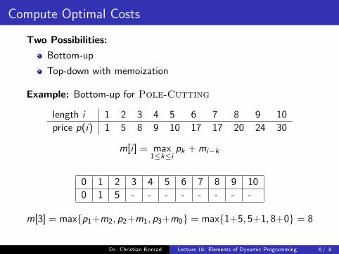
Compute Optimal Costs
Two Possibilities:
Bottom-up
Top-down with memoization
Example: Bottom-up for Pole-Cutting
length i 1 2 3 4 5 6 7 8 9 10
price p(i) 1 5 8 9 10 17 17 20 24 30
m[i ] = max1≤k≤i
pk + mi−k
0 1 2 3 4 5 6 7 8 9 10
0 1 5 8 - - - - - - -
m[3] = max{p1+m2, p2+m1, p3+m0} = max{1+5, 5+1, 8+0} = 8
Dr. Christian Konrad Lecture 18: Elements of Dynamic Programming 6 / 8
Compute Optimal Costs
Two Possibilities:
Bottom-up
Top-down with memoization
Example: Bottom-up for Pole-Cutting
length i 1 2 3 4 5 6 7 8 9 10
price p(i) 1 5 8 9 10 17 17 20 24 30
m[i ] = max1≤k≤i
pk + mi−k
0 1 2 3 4 5 6 7 8 9 10
0 1 5 8 - - - - - - -
m[4] = max{p1 +m3, p2 +m2, p3 +m1, p4 +m0} = max{1 + 8, 5 +5, 8 + 1, 9} = 10
Dr. Christian Konrad Lecture 18: Elements of Dynamic Programming 6 / 8
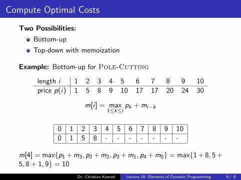
Compute Optimal Costs
Two Possibilities:
Bottom-up
Top-down with memoization
Example: Bottom-up for Pole-Cutting
length i 1 2 3 4 5 6 7 8 9 10
price p(i) 1 5 8 9 10 17 17 20 24 30
m[i ] = max1≤k≤i
pk + mi−k
0 1 2 3 4 5 6 7 8 9 10
0 1 5 8 10 - - - - - -
m[4] = max{p1 +m3, p2 +m2, p3 +m1, p4 +m0} = max{1 + 8, 5 +5, 8 + 1, 9} = 10
Dr. Christian Konrad Lecture 18: Elements of Dynamic Programming 6 / 8
Compute Optimal Costs
Two Possibilities:
Bottom-up
Top-down with memoization
Example: Bottom-up for Pole-Cutting
length i 1 2 3 4 5 6 7 8 9 10
price p(i) 1 5 8 9 10 17 17 20 24 30
m[i ] = max1≤k≤i
pk + mi−k
0 1 2 3 4 5 6 7 8 9 10
0 1 5 8 10 - - - - - -
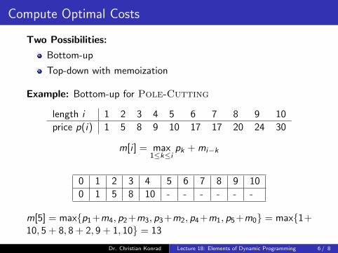
m[5] = max{p1+m4, p2+m3, p3+m2, p4+m1, p5+m0} = max{1+10, 5 + 8, 8 + 2, 9 + 1, 10} = 13
Dr. Christian Konrad Lecture 18: Elements of Dynamic Programming 6 / 8
Compute Optimal Costs
Two Possibilities:
Bottom-up
Top-down with memoization
Example: Bottom-up for Pole-Cutting
length i 1 2 3 4 5 6 7 8 9 10
price p(i) 1 5 8 9 10 17 17 20 24 30
m[i ] = max1≤k≤i
pk + mi−k
0 1 2 3 4 5 6 7 8 9 10
0 1 5 8 10 13 - - - - -
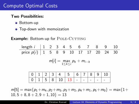
m[5] = max{p1+m4, p2+m3, p3+m2, p4+m1, p5+m0} = max{1+10, 5 + 8, 8 + 2, 9 + 1, 10} = 13
Dr. Christian Konrad Lecture 18: Elements of Dynamic Programming 6 / 8

Compute Optimal Costs
Two Possibilities:
Bottom-up
Top-down with memoization
Example: Bottom-up for Pole-Cutting
length i 1 2 3 4 5 6 7 8 9 10
price p(i) 1 5 8 9 10 17 17 20 24 30
m[i ] = max1≤k≤i
pk + mi−k
0 1 2 3 4 5 6 7 8 9 10
0 1 5 8 10 13 - - - - -
. . .
Dr. Christian Konrad Lecture 18: Elements of Dynamic Programming 6 / 8
Compute Optimal Costs
Two Possibilities:
Bottom-up
Top-down with memoization
Example: Bottom-up for Pole-Cutting
length i 1 2 3 4 5 6 7 8 9 10
price p(i) 1 5 8 9 10 17 17 20 24 30
m[i ] = max1≤k≤i
pk + mi−k
0 1 2 3 4 5 6 7 8 9 10
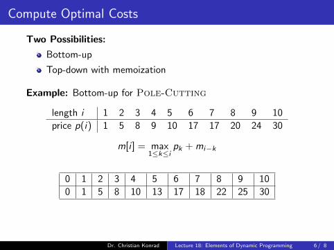
0 1 5 8 10 13 17 18 22 25 30
Dr. Christian Konrad Lecture 18: Elements of Dynamic Programming 6 / 8
Compute Optimal Costs
Two Possibilities:
Bottom-up
Top-down with memoization
Example: Bottom-up for Pole-Cutting
length i 1 2 3 4 5 6 7 8 9 10
price p(i) 1 5 8 9 10 17 17 20 24 30
m[i ] = max1≤k≤i
pk + mi−k
0 1 2 3 4 5 6 7 8 9 10
0 1 5 8 10 13 17 18 22 25 30
The maximum revenue obtainable for a pole of length 10 is 30
Dr. Christian Konrad Lecture 18: Elements of Dynamic Programming 6 / 8
Compute Optimal Costs
Two Possibilities:
Bottom-up
Top-down with memoization
Example: Bottom-up for Pole-Cutting
length i 1 2 3 4 5 6 7 8 9 10
price p(i) 1 5 8 9 10 17 17 20 24 30
m[i ] = max1≤k≤i
pk + mi−k
0 1 2 3 4 5 6 7 8 9 10
0 1 5 8 10 13 17 18 22 25 30
But how can we find out how to cut the pole?
Dr. Christian Konrad Lecture 18: Elements of Dynamic Programming 6 / 8
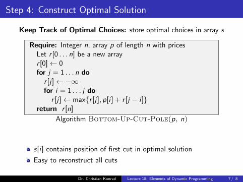
Step 4: Construct Optimal Solution
Keep Track of Optimal Choices: store optimal choices in array s
Require: Integer n, array p of length n with pricesLet r [0 . . . n] be a new arrayr [0]← 0for j = 1 . . . n dor [j ]← −∞for i = 1 . . . j do
r [j ]← max{r [j ], p[i ] + r [j − i ]}return r [n]
Algorithm Bottom-Up-Cut-Pole(p, n)
s[i ] contains position of first cut in optimal solution
Easy to reconstruct all cuts
Dr. Christian Konrad Lecture 18: Elements of Dynamic Programming 7 / 8
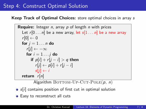
Step 4: Construct Optimal Solution
Keep Track of Optimal Choices: store optimal choices in array s
Require: Integer n, array p of length n with pricesLet r [0 . . . n] be a new array, let s[1 . . . n] be a new arrayr [0]← 0for j = 1 . . . n dor [j ]← −∞for i = 1 . . . j do
if p[i ] + r [j − i ] > q thenr [j ]← p[i ] + r [j − i ]s[j ]← i
return r [n]
Algorithm Bottom-Up-Cut-Pole(p, n)
s[i ] contains position of first cut in optimal solution
Easy to reconstruct all cuts
Dr. Christian Konrad Lecture 18: Elements of Dynamic Programming 7 / 8
Subproblem Graph and Runtime
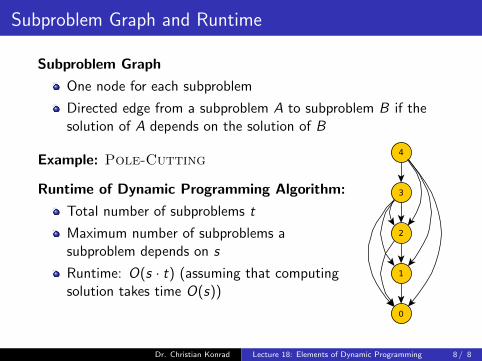
Subproblem Graph
One node for each subproblem
Directed edge from a subproblem A to subproblem B if thesolution of A depends on the solution of B
Example: Pole-Cutting
Runtime of Dynamic Programming Algorithm:
Total number of subproblems t
Maximum number of subproblems asubproblem depends on s
Runtime: O(s · t) (assuming that computingsolution takes time O(s))
Dr. Christian Konrad Lecture 18: Elements of Dynamic Programming 8 / 8