Lecture 16 Image Segmentation

1. The basic concepts of segmentation

2. Point, line, edge detection

3. Thresh holding

4. Region-based segmentation

5. Segmentation with Matlab

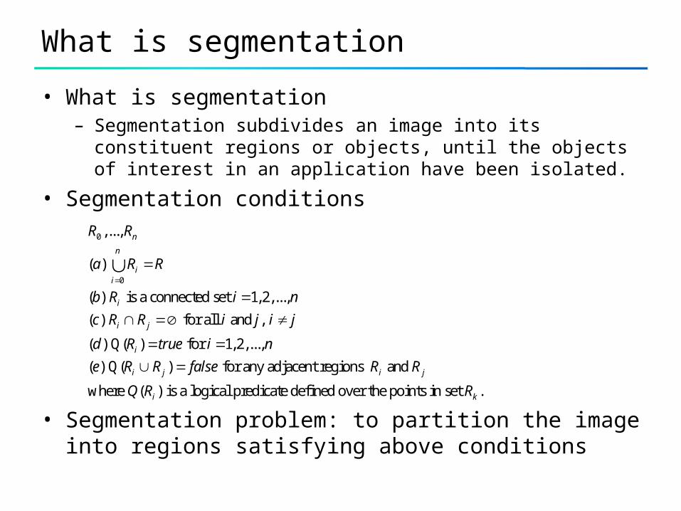
What is segmentation

• What is segmentation– Segmentation subdivides an image into its constituent regions or

objects, until the objects of interest in an application have been isolated.

• Segmentation conditions

• Segmentation problem: to partition the image into regions satisfying above conditions

0

0

,...,

( )

( ) is a connected set 1, 2,...,

( ) for all and ,

( ) Q( ) for 1,2,...,

( ) Q( ) for any adjacent regions and

where ( ) is a logical

n

n

ii

i

i j

i

i j i j

i

R R

a R R

b R i n

c R R i j i j

d R true i n

e R R false R R

Q R

predicate defined over the points in set . kR

Two principal approaches

• Edge-based segmentation– partition an image based on abrupt changes in intensity (edges)

• Region-based segmentation– partition an image into regions that are similar according to a set

of predefined criteria.

4

Detection of Discontinuities

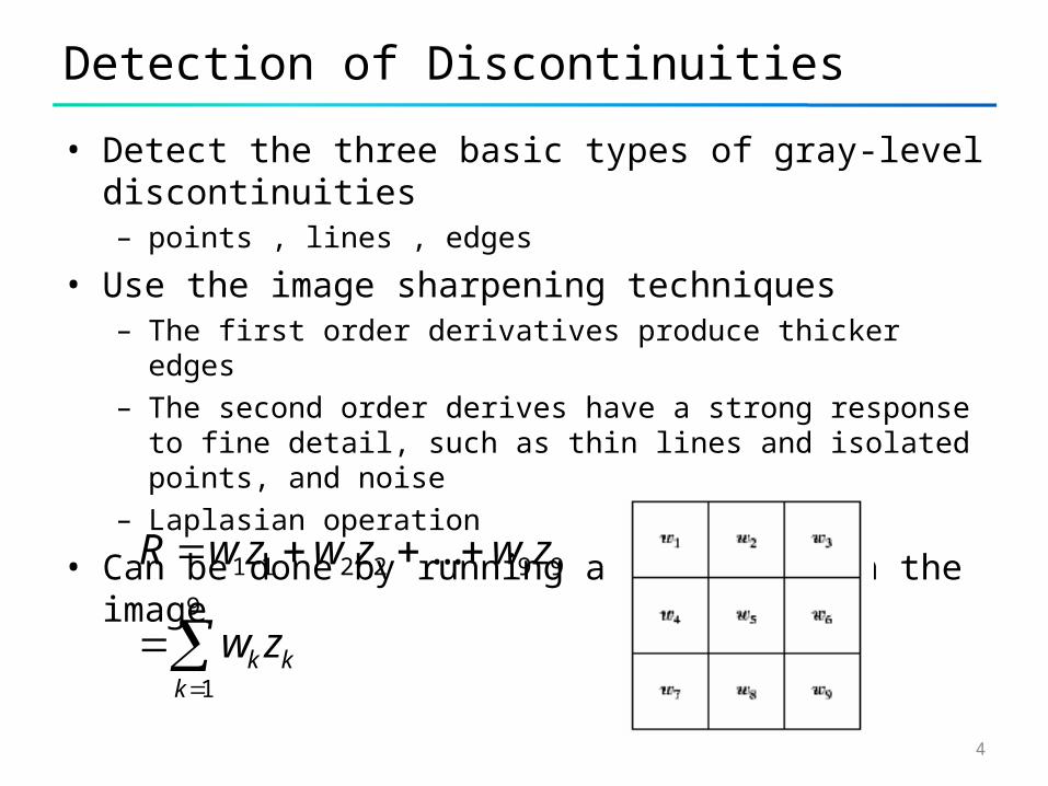
• Detect the three basic types of gray-level discontinuities– points , lines , edges

• Use the image sharpening techniques– The first order derivatives produce thicker edges– The second order derives have a strong response to fine detail,

such as thin lines and isolated points, and noise– Laplasian operation

• Can be done by running a mask through the image

1 1 2 2 9 9

9

1

...

k kk

R w z w z w z

w z

5

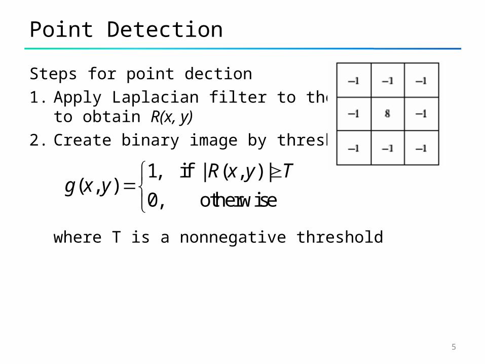
Point Detection

Steps for point dection

1. Apply Laplacian filter to the imageto obtain R(x, y)

2. Create binary image by threshold

where T is a nonnegative threshold

1, if | ( , ) |( , )

0, otherwise

R x y Tg x y

6

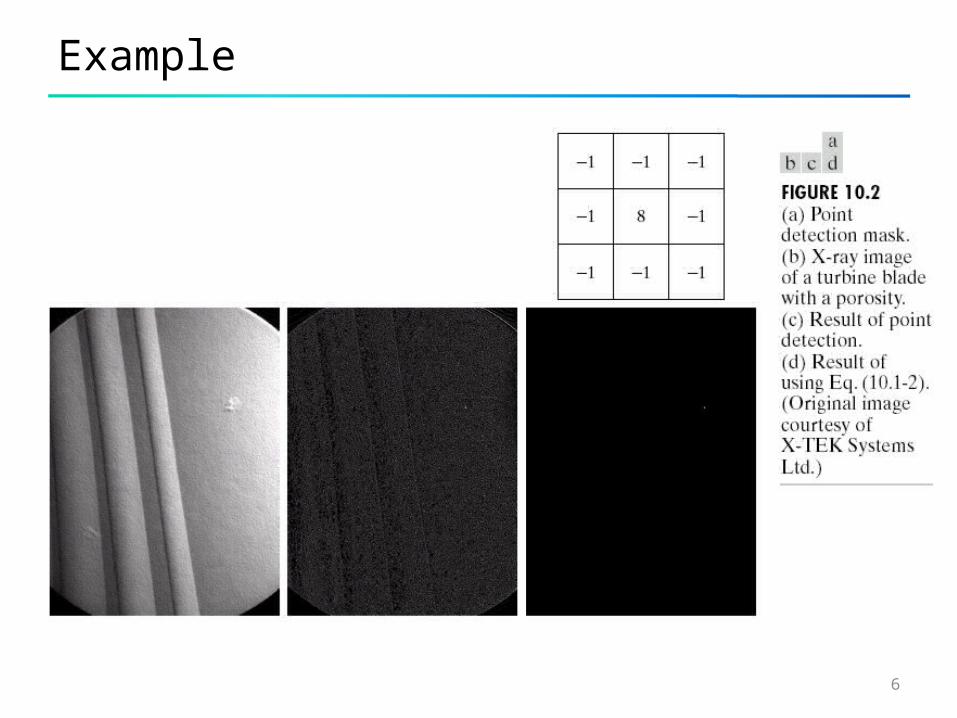
Example

7

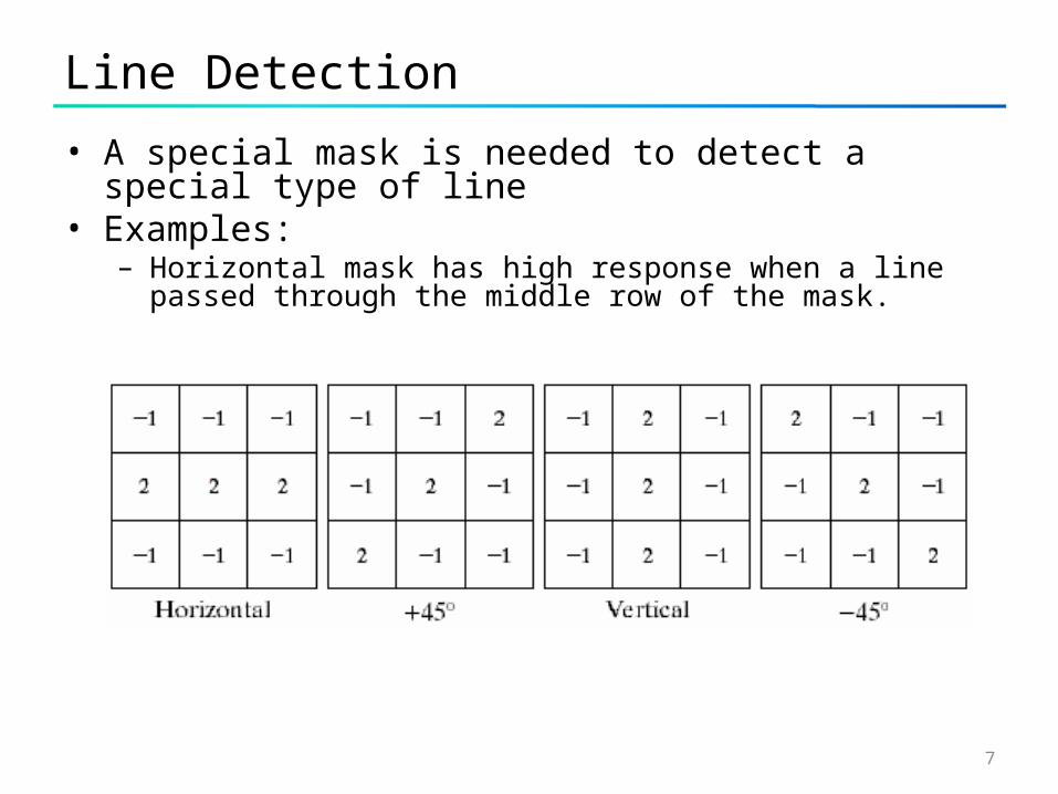
Line Detection

• A special mask is needed to detect a special type of line• Examples:

– Horizontal mask has high response when a line passed through the middle row of the mask.

8

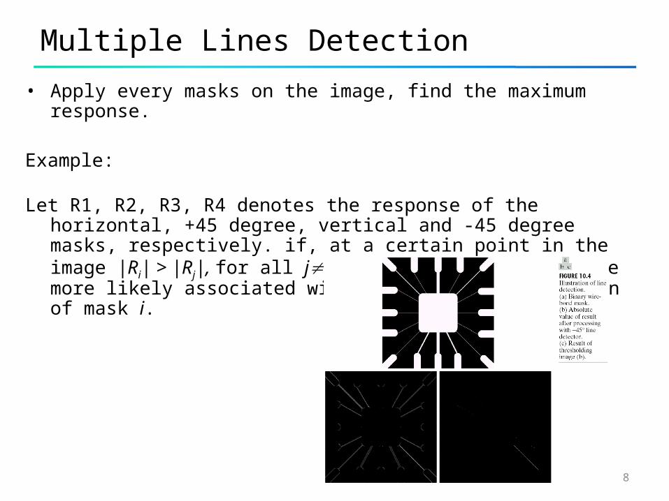
Multiple Lines Detection

• Apply every masks on the image, find the maximum response.

Example:

Let R1, R2, R3, R4 denotes the response of the horizontal, +45 degree, vertical and -45 degree masks, respectively. if, at a certain point in the image |Ri| > |Rj|, for all ji, that point is said to be more likely associated with a line in the direction of mask i.

9

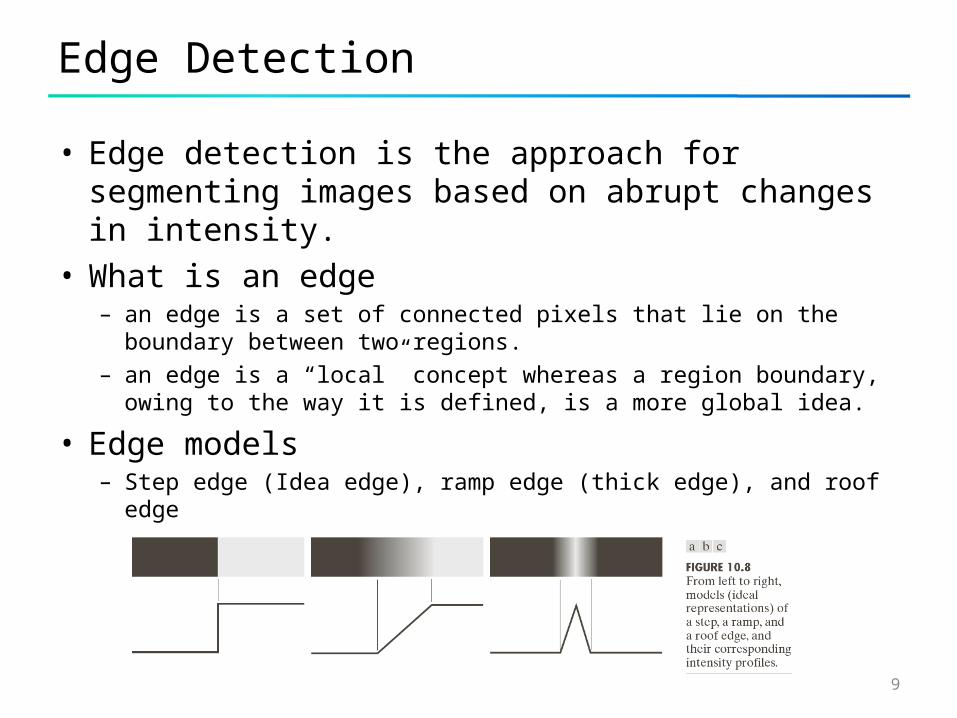
Edge Detection

• Edge detection is the approach for segmenting images based on abrupt changes in intensity.

• What is an edge– an edge is a set of connected pixels that lie on the boundary

between two regions.– an edge is a “local” concept whereas a region boundary, owing

to the way it is defined, is a more global idea.

• Edge models– Step edge (Idea edge), ramp edge (thick edge), and roof edge

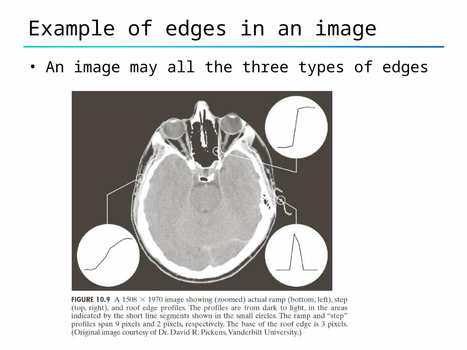
Example of edges in an image

• An image may all the three types of edges

11

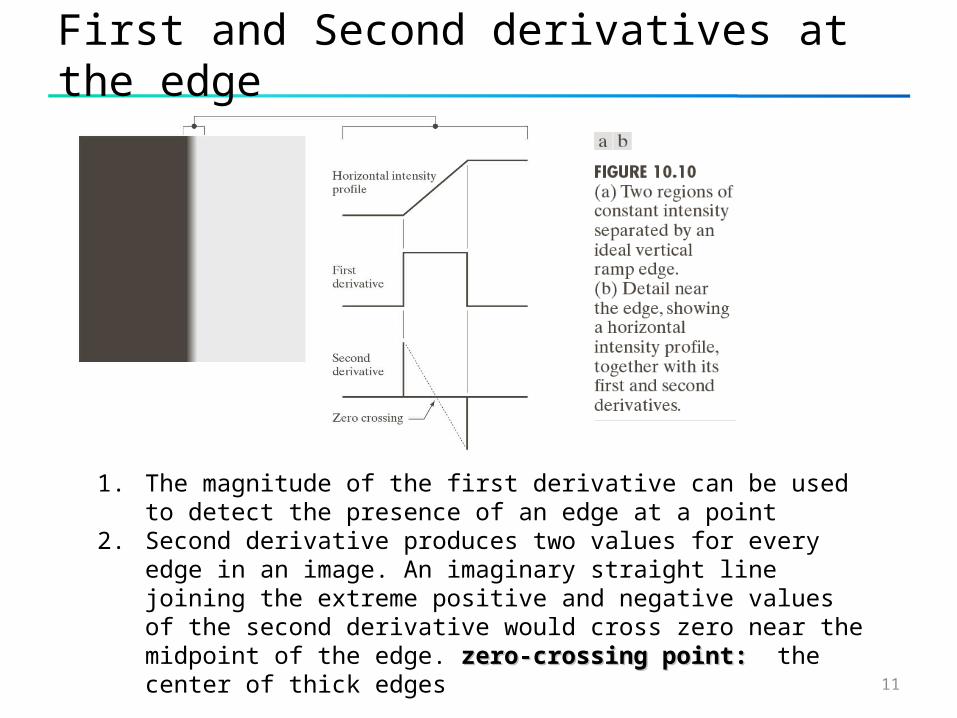
First and Second derivatives at the edge

1. The magnitude of the first derivative can be used to detect the presence of an edge at a point

2. Second derivative produces two values for every edge in an image. An imaginary straight line joining the extreme positive and negative values of the second derivative would cross zero near the midpoint of the edge. zero-crossing point: zero-crossing point: the center of thick edges

12

Noise Images

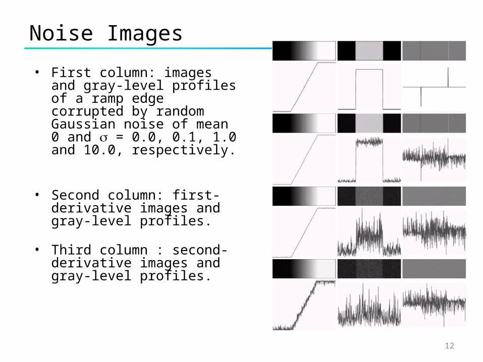
• First column: images and gray-level profiles of a ramp edge corrupted by random Gaussian noise of mean 0 and = 0.0, 0.1, 1.0 and 10.0, respectively.

• Second column: first-derivative images and gray-level profiles.

• Third column : second-derivative images and gray-level profiles.

13

Steps in edge detection

1. Image smoothing for noise reduction

2. Detection of edge points. Points on an edge

3. Edge localization

14

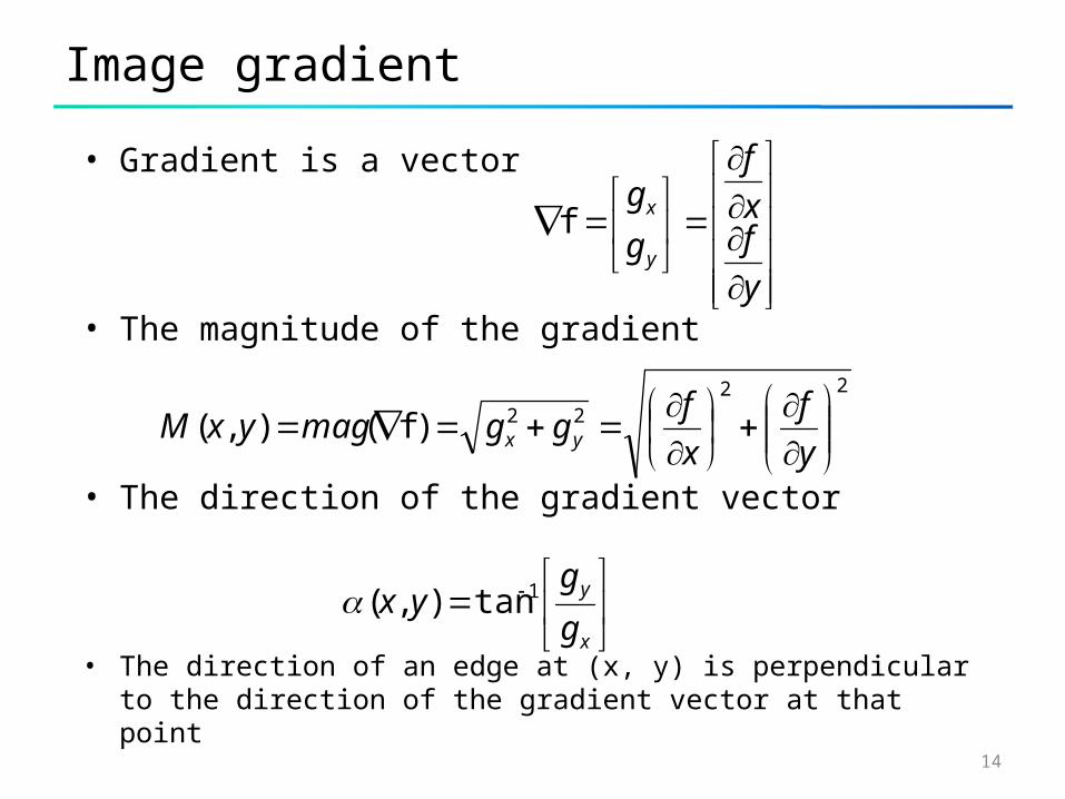
Image gradient

• Gradient is a vector

• The magnitude of the gradient

• The direction of the gradient vector

• The direction of an edge at (x, y) is perpendicular to the direction of the gradient vector at that point

y

fx

f

g

g

y

xf

2222)f(),(

y

f

x

fggmagyxM yx

x

y

g

gyx 1tan),(

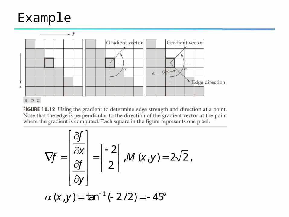
Example

1

2, ( , ) 2 2,

2

( , ) tan ( 2 / 2) 45o

f

xf M x y

f

y

x y

16

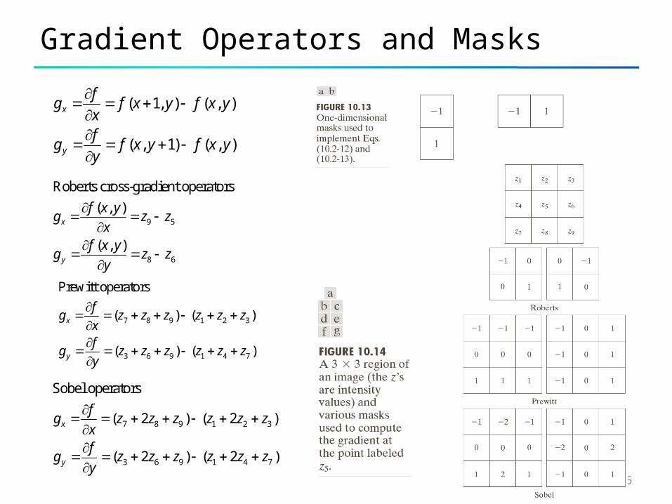
Gradient Operators and Masks

( 1, ) ( , )

( , 1) ( , )

x

y

fg f x y f x y

xf

g f x y f x yy

9 5

8 6

Roberts cross-gradient operators

( , )

( , )

x

y

f x yg z z

xf x y

g z zy

7 8 9 1 2 3

3 6 9 1 4 7

Prewitt operators

( ) ( )

( ) ( )

x

y

fg z z z z z z

xf

g z z z z z zy

7 8 9 1 2 3

3 6 9 1 4 7

Sobel operators

( 2 ) ( 2 )

( 2 ) ( 2 )

x

y

fg z z z z z z

xf

g z z z z z zy

17

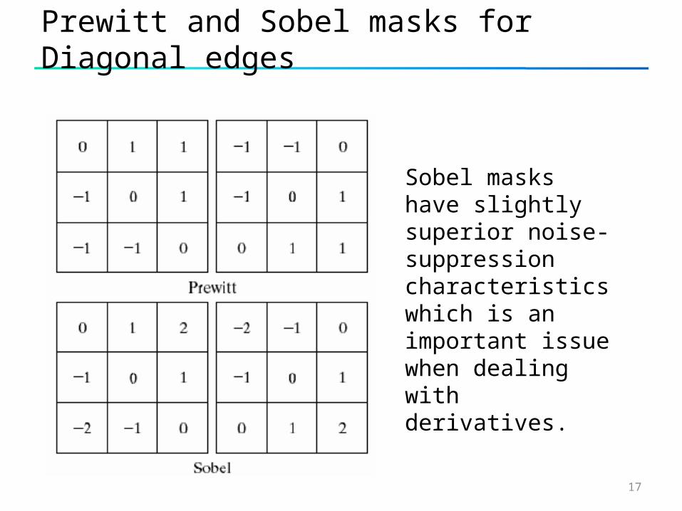
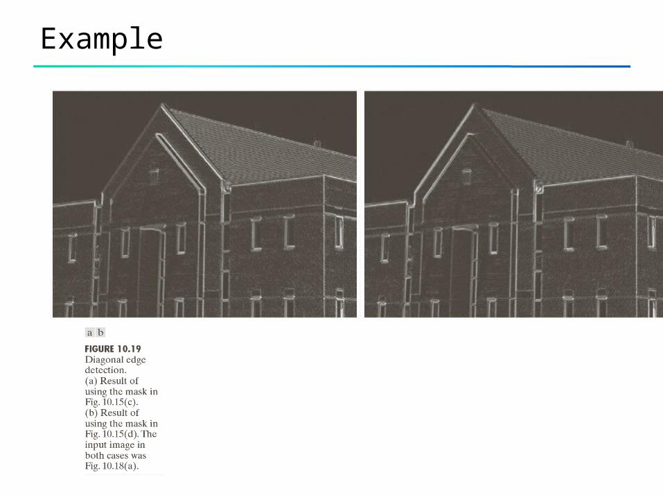
Prewitt and Sobel masks for Diagonal edges

Sobel masks have slightly superior noise-suppression characteristics which is an important issue when dealing with derivatives.

18

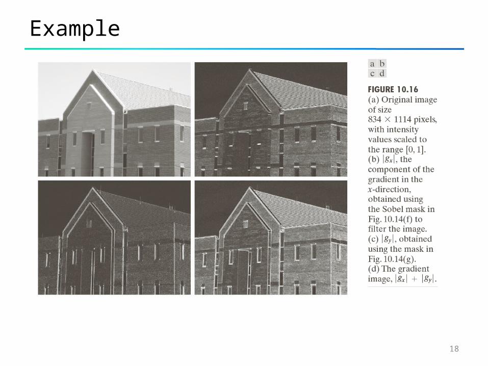
Example

Example

20

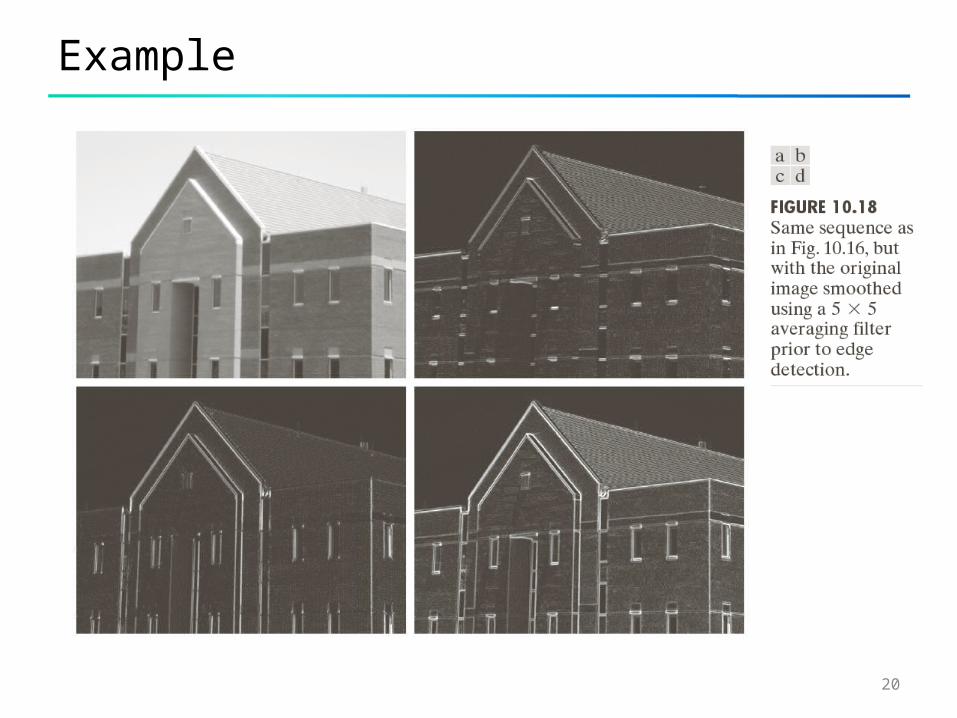
Example

Example

22

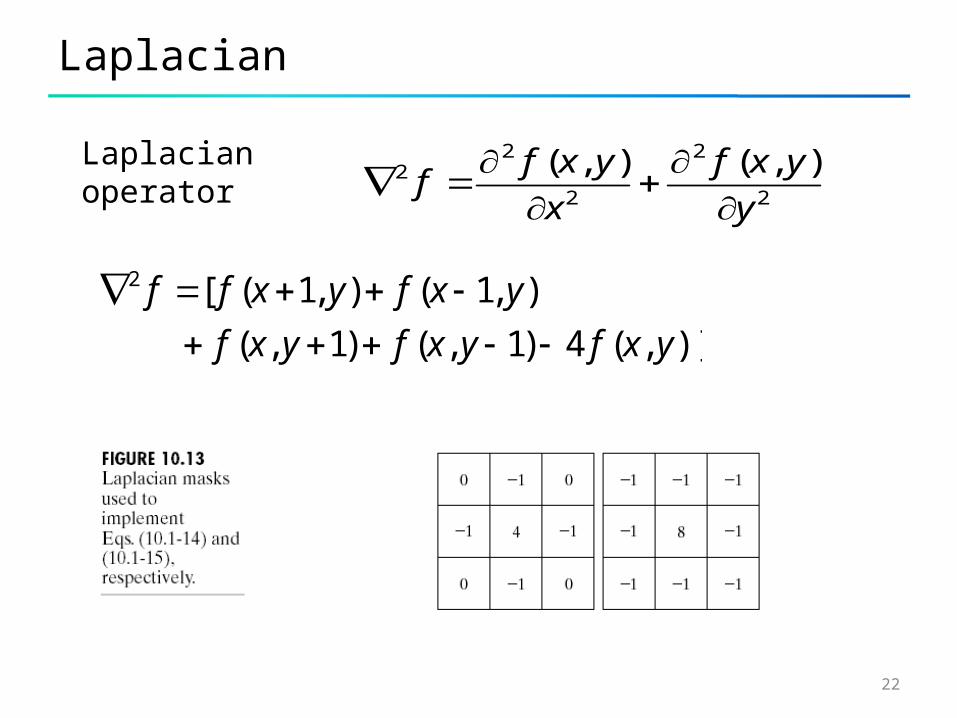
Laplacian

2

2

2

22 ),(),(

y

yxf

x

yxff

Laplacian operator

)],(4)1,()1,(

),1(),1([2

yxfyxfyxf

yxfyxff

23

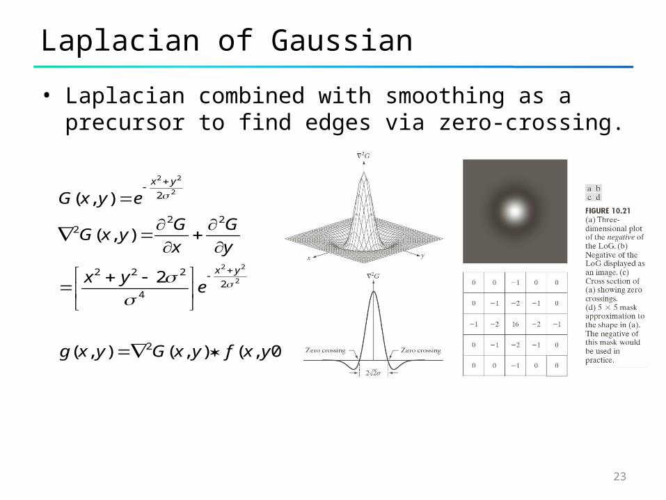
Laplacian of Gaussian

• Laplacian combined with smoothing as a precursor to find edges via zero-crossing.

0,(),(),(

2

),(

),(

2

24

222

222

2

2

22

2

22

yxfyxGyxg

eyx

y

G

x

GyxG

eyxG

yx

yx

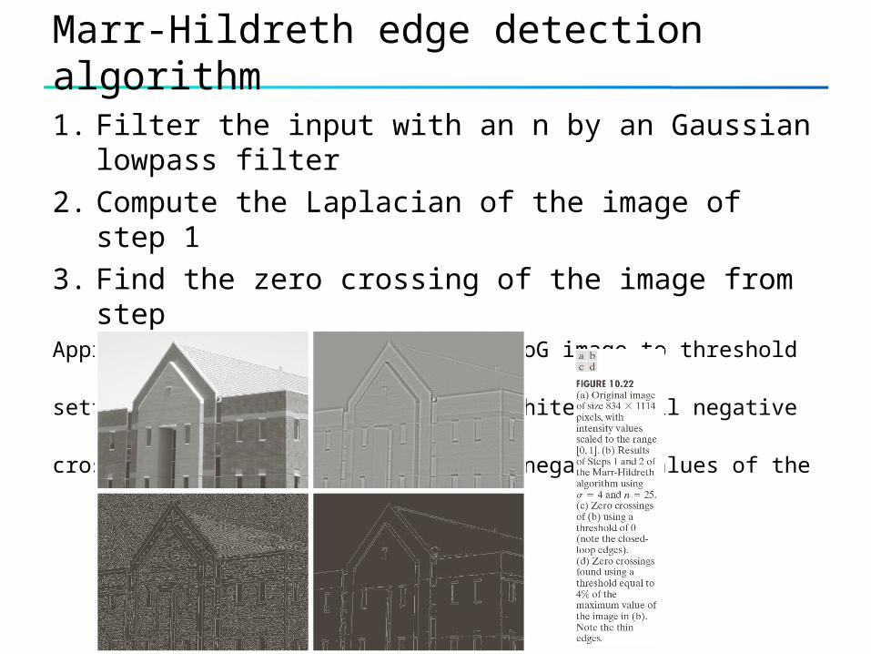
Marr-Hildreth edge detection algorithm

1. Filter the input with an n by an Gaussian lowpass filter

2. Compute the Laplacian of the image of step 1

3. Find the zero crossing of the image from step Approximate the zero crossing from LoG image to threshold the LoG image by

setting all its positive values to white and all negative values to black. the zero

crossing occur between positive and negative values of the thresholded LoG.

25

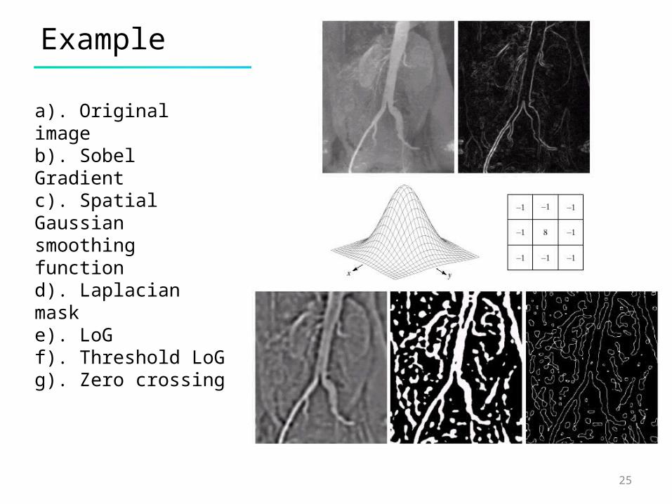
Example

a). Original imageb). Sobel Gradientc). Spatial Gaussian smoothing functiond). Laplacian maske). LoGf). Threshold LoGg). Zero crossing

26

Zero crossing vs. Gradient

• Attractive– Zero crossing produces thinner edges– Noise reduction

• Drawbacks– Zero crossing creates closed loops. (spaghetti effect)– sophisticated computation.

• Gradient is more frequently used.

27

Edge Linking and Boundary Detection

• An edge detection algorithm are followed by linking procedures to assemble edge pixels into meaningful edges.

• Basic approaches– Local Processing– Global Processing via the Hough Transform– Global Processing via Graph-Theoretic Techniques

28

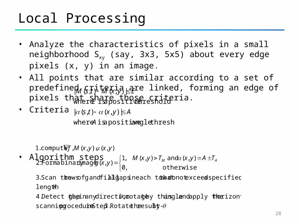
Local Processing

• Analyze the characteristics of pixels in a small neighborhood Sxy (say, 3x3, 5x5) about every edge pixels (x, y) in an image.

• All points that are similar according to a set of predefined criteria are linked, forming an edge of pixels that share those criteria.

• Criteria

• Algorithm steps

thresholdangle positive a is where

|),(),(|

thresholdpositive a is where

|),(),(|

A

Ayxts

E

EyxMtsM

-by result theRotate 3. Stepin procedure scanning

horizontal apply the and angle by this g rotate ,direction any in gap Detect the 4.

Klength

specified a exceednot do that ineach tow gaps all fill and g of rows Scan the .3

otherwise,0

),( and ),(,1),( imagebinary a Form .2

),(),,(, compute .1

AM TAyxTyxMyxg

yxyxMf

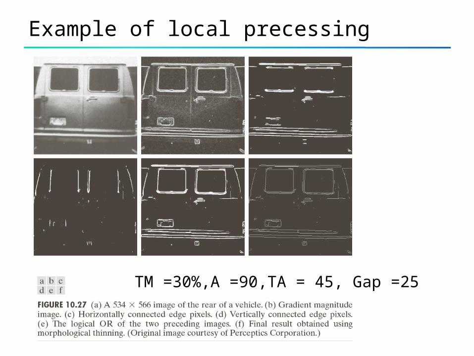
Example of local precessing

TM =30%,A =90,TA = 45, Gap =25

30

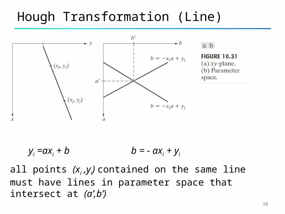
Hough Transformation (Line)

yi =axi + b b = - axi + yi

all points (xi ,yi) contained on the same line must have lines in parameter space that intersect at (a’,b’)

31

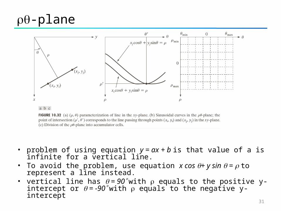
-plane

• problem of using equation y = ax + b is that value of a is infinite for a vertical line.

• To avoid the problem, use equation x cos + y sin = to represent a line instead.

• vertical line has = 90 with equals to the positive y-intercept or = -90 with equals to the negative y-intercept

33

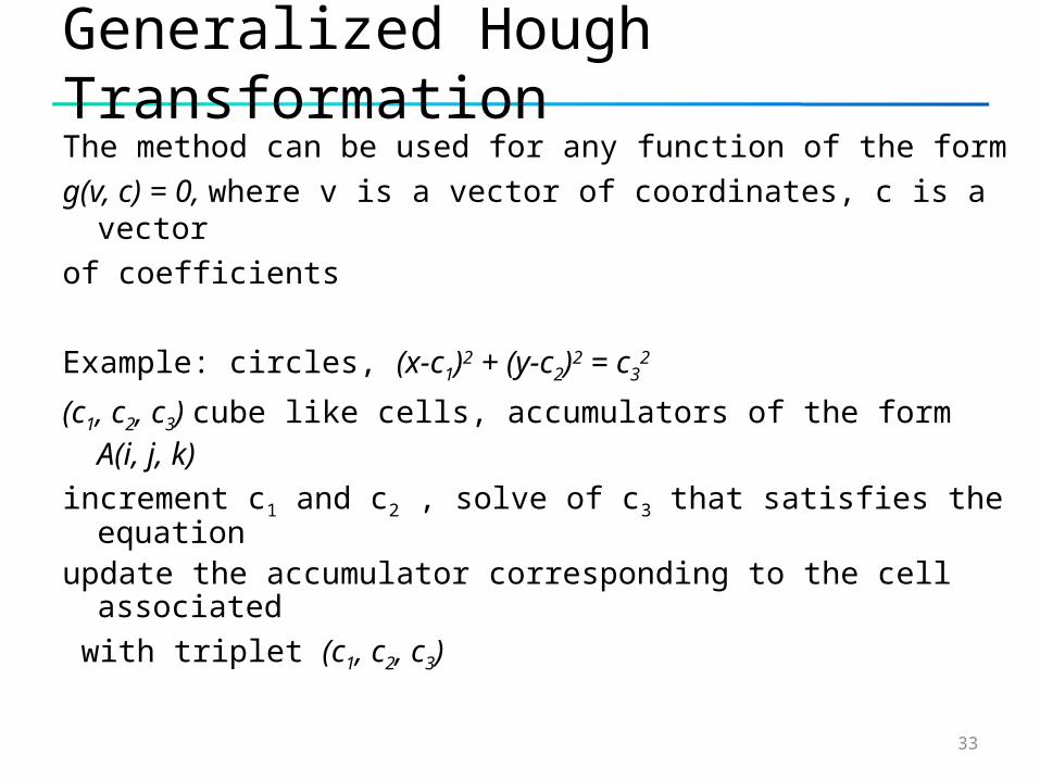
Generalized Hough TransformationThe method can be used for any function of the form

g(v, c) = 0, where v is a vector of coordinates, c is a vector

of coefficients

Example: circles, (x-c1)2 + (y-c2)2 = c32

(c1, c2, c3) cube like cells, accumulators of the form A(i, j, k)

increment c1 and c2 , solve of c3 that satisfies the equationupdate the accumulator corresponding to the cell associated

with triplet (c1, c2, c3)

34

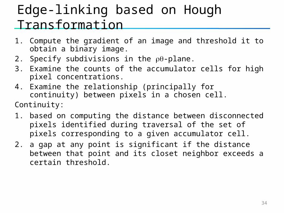
Edge-linking based on Hough Transformation

1. Compute the gradient of an image and threshold it to obtain a binary image.

2. Specify subdivisions in the -plane.3. Examine the counts of the accumulator cells for high pixel

concentrations.4. Examine the relationship (principally for continuity) between

pixels in a chosen cell.Continuity:

1. based on computing the distance between disconnected pixels identified during traversal of the set of pixels corresponding to a given accumulator cell.

2. a gap at any point is significant if the distance between that point and its closet neighbor exceeds a certain threshold.

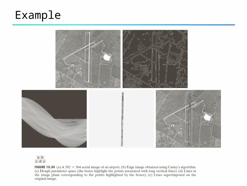
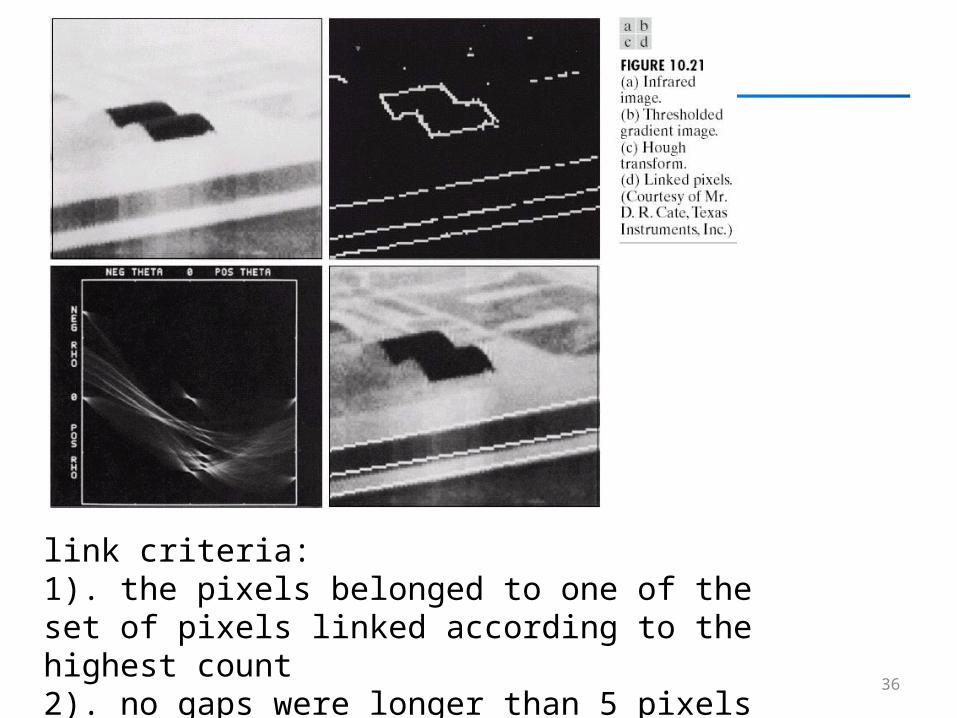
Example

36

link criteria:1). the pixels belonged to one of the set of pixels linked according to the highest count2). no gaps were longer than 5 pixels

Image Segmentation II

1. Threshold

2. Region-based segmentation

3. Segmentation using watersheds

4. Segmentation with Matlab

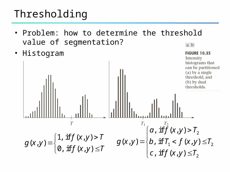
Thresholding

• Problem: how to determine the threshold value of segmentation?

• Histogram

1, if ( , )( , )

0, if ( , )

f x y Tg x y

f x y T

2

1 2

2

, if ( , )

( , ) , if ( , )

, if ( , )

a f x y T

g x y b T f x y T

c f x y T

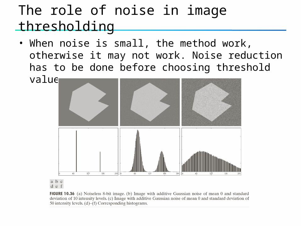
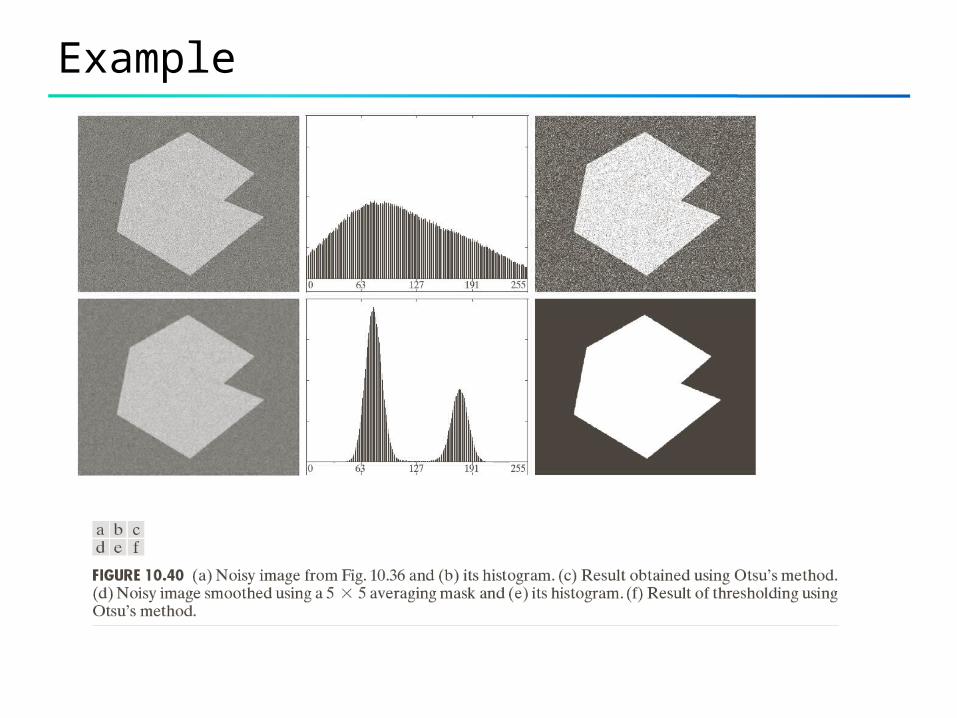
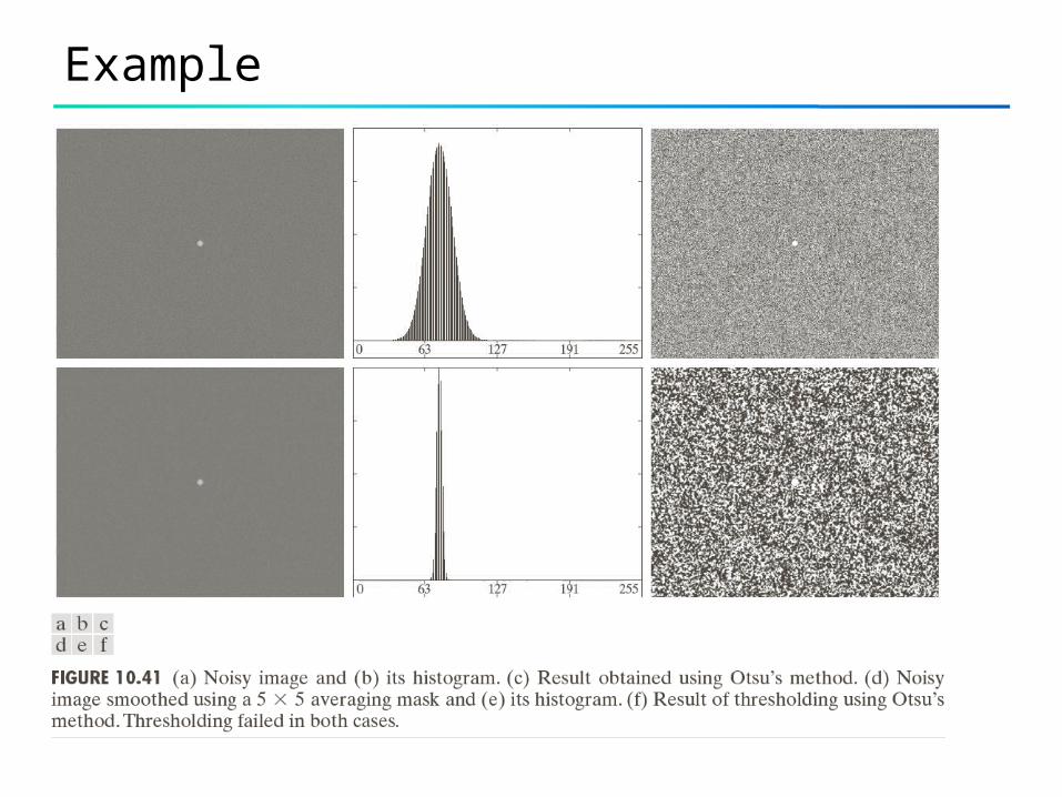
The role of noise in image thresholding

• When noise is small, the method work, otherwise it may not work. Noise reduction has to be done before choosing threshold value

40

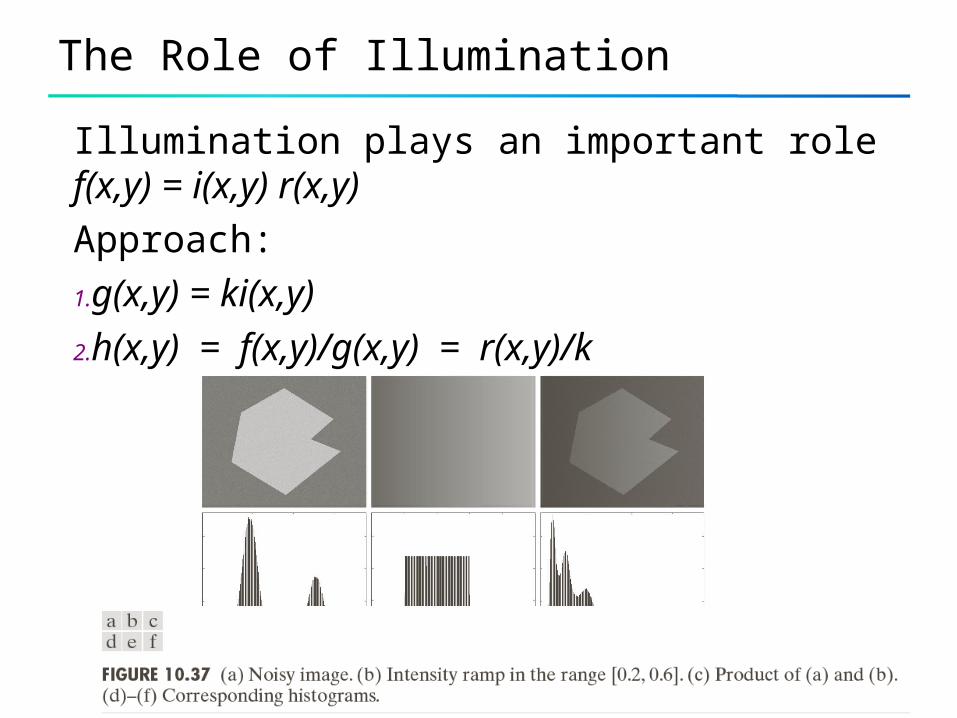
The Role of Illumination

Illumination plays an important rolef(x,y) = i(x,y) r(x,y)

Approach:

1.g(x,y) = ki(x,y)

2.h(x,y) = f(x,y)/g(x,y) = r(x,y)/k

41

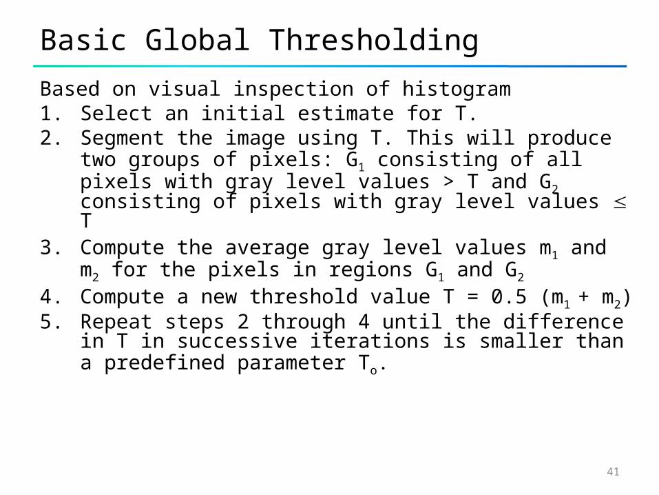
Basic Global Thresholding

Based on visual inspection of histogram1. Select an initial estimate for T.2. Segment the image using T. This will produce two

groups of pixels: G1 consisting of all pixels with gray level values > T and G2 consisting of pixels with gray level values T

3. Compute the average gray level values m1 and m2 for the pixels in regions G1 and G2

4. Compute a new threshold value T = 0.5 (m1 + m2)5. Repeat steps 2 through 4 until the difference in T in

successive iterations is smaller than a predefined parameter To.

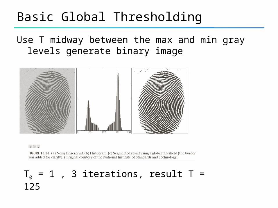
Basic Global Thresholding

Use T midway between the max and min gray levels generate binary image

T0 = 1 , 3 iterations, result T = 125

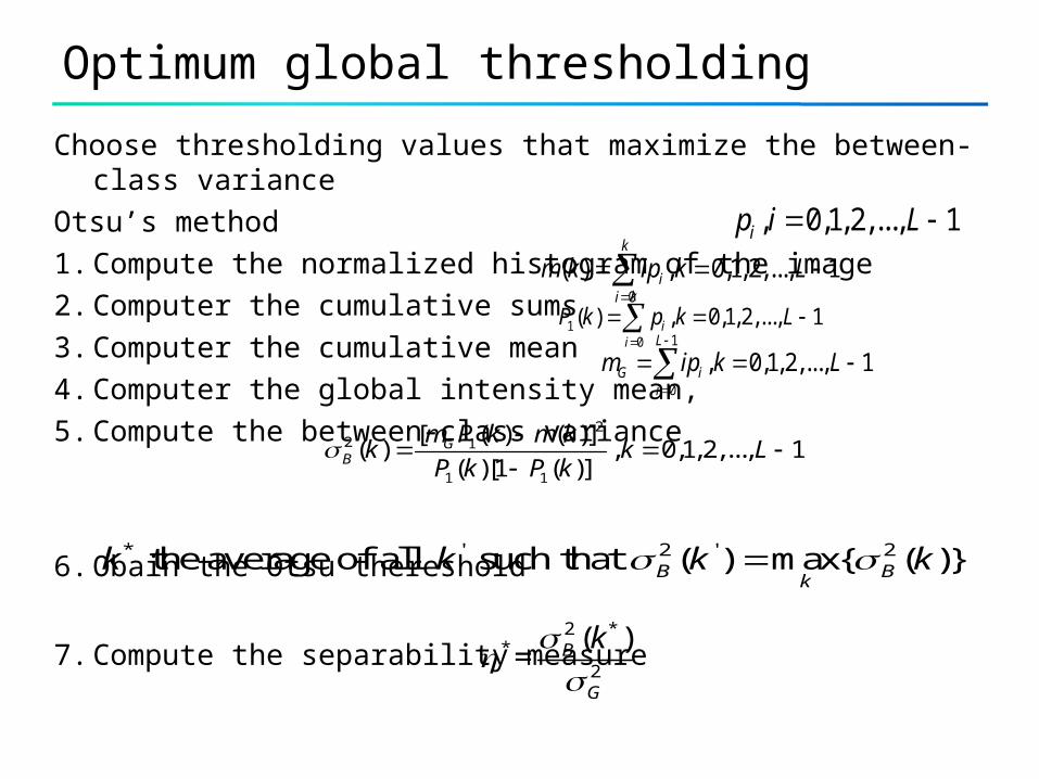
Optimum global thresholding

Choose thresholding values that maximize the between-class variance

Otsu’s method

1. Compute the normalized histogram of the image

2. Computer the cumulative sums

3. Computer the cumulative mean

4. Computer the global intensity mean,

5. Compute the between-class variance

6. Obain the Otsu thereshold

7. Compute the separability measure

, 0,1,2,..., 1ip i L

10

( ) , 0,1, 2,..., 1k

ii

P k p k L

0

( ) , 0,1,2,..., 1k

ii

m k ip k L

1

0

, 0,1,2,..., 1L

G ii

m ip k L

2

2 1

1 1

[ ( ) ( )]( ) , 0,1,2,..., 1

( )[1 ( )]G

B

m P k m kk k L

P k P k

* ' 2 ' 2 the average of all such that ( ) max{ ( )}B Bk

k k k k

2 **

2

( )= B

G

k

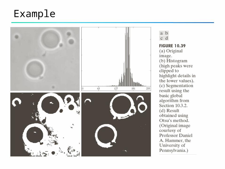
Example

Example

Example

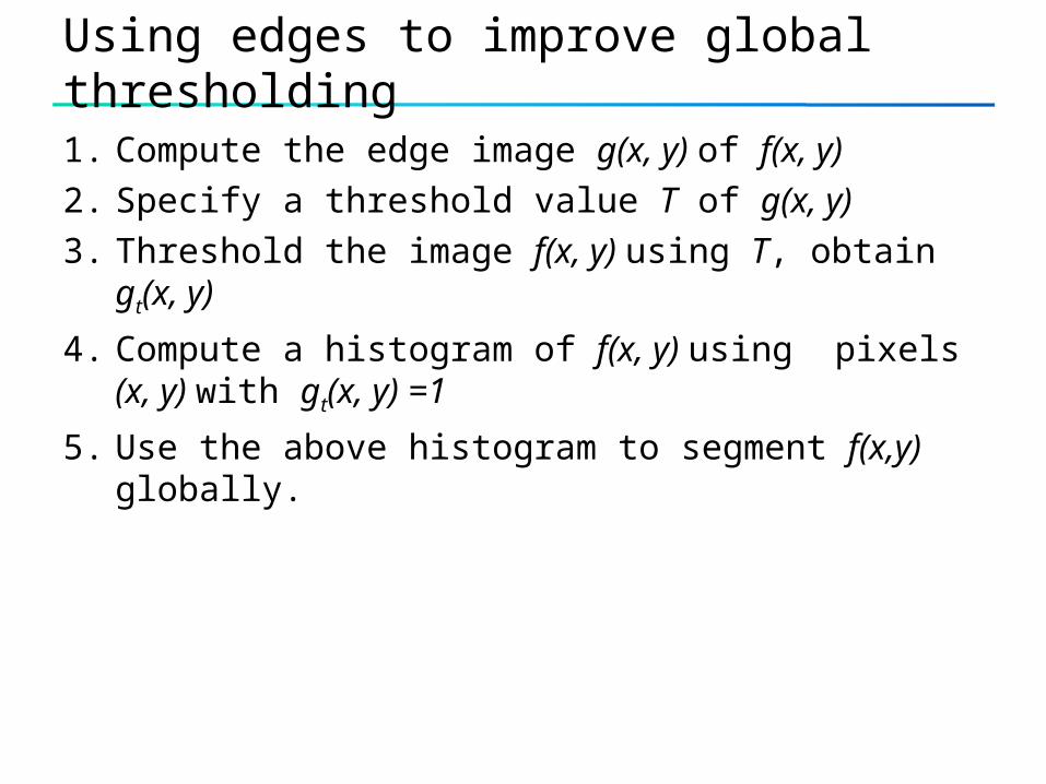
Using edges to improve global thresholding

1. Compute the edge image g(x, y) of f(x, y)

2. Specify a threshold value T of g(x, y)

3. Threshold the image f(x, y) using T, obtain gt(x, y)

4. Compute a histogram of f(x, y) using pixels (x, y) with gt(x, y) =1

5. Use the above histogram to segment f(x,y) globally.

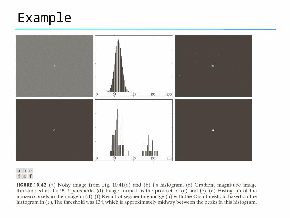
Example

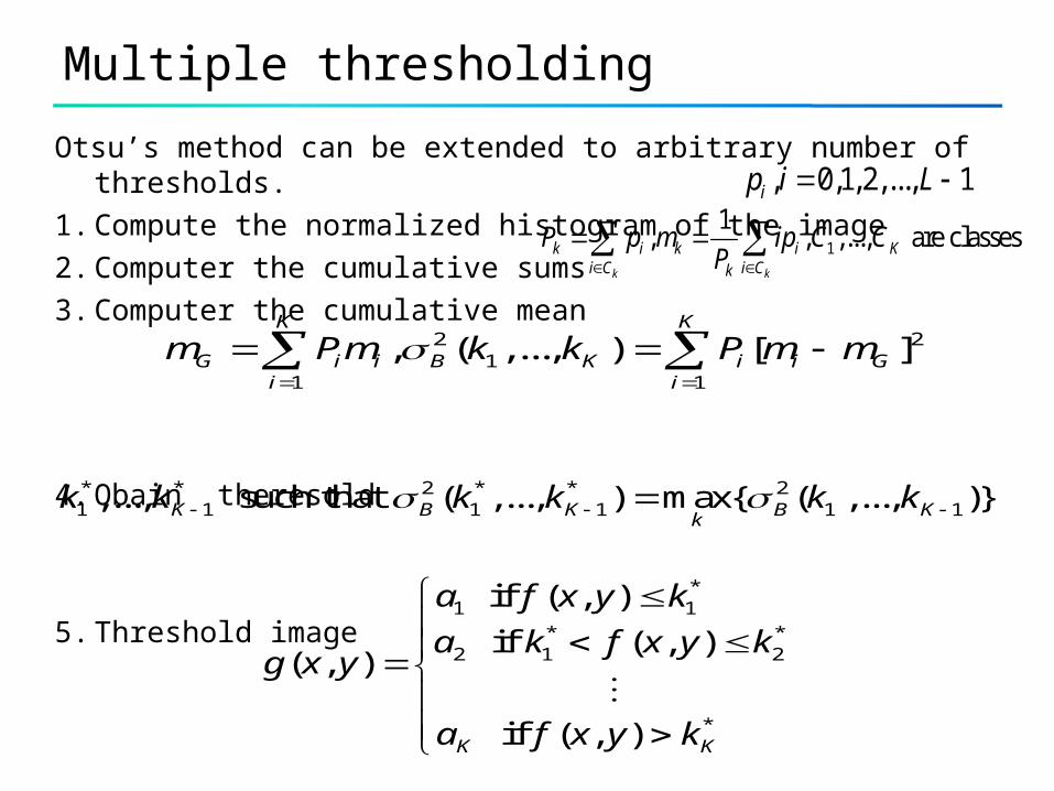
Multiple thresholding

Otsu’s method can be extended to arbitrary number of thresholds.

1. Compute the normalized histogram of the image

2. Computer the cumulative sums

3. Computer the cumulative mean

4. Obain theresold

5. Threshold image

, 0,1, 2,..., 1ip i L

1

1, , ,..., are classes

k k

k i k i Ki C i Ck

P p m ip C CP

2 21

1 1

, ( ,..., ) [ ]K K

G i i B K i i Gi i

m Pm k k P m m

* * 2 * * 21 1 1 1 1 1,..., such that ( ,..., ) max{ ( ,..., )}K B K B K

kk k k k k k

*1 1

* *2 1 2

*

if ( , )

if ( , )( , )

if ( , ) K K

a f x y k

a k f x y kg x y

a f x y k

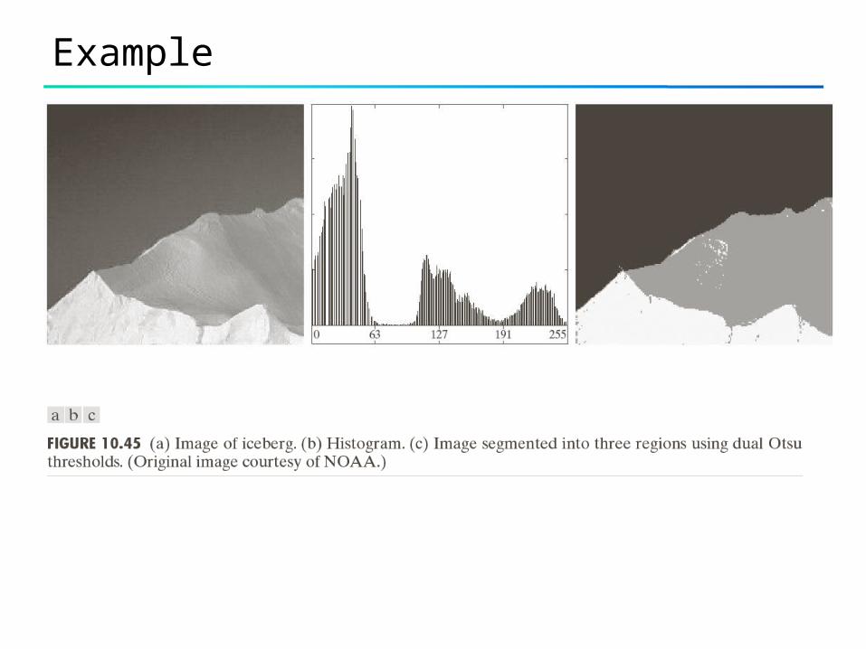
Example

51

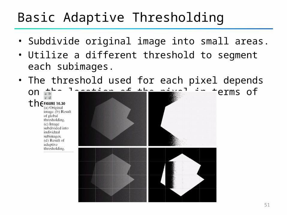
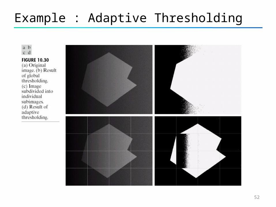
Basic Adaptive Thresholding

• Subdivide original image into small areas.• Utilize a different threshold to segment each subimages.• The threshold used for each pixel depends on the

location of the pixel in terms of the subimages.

52

Example : Adaptive Thresholding

53

2. Region-Based Segmentation

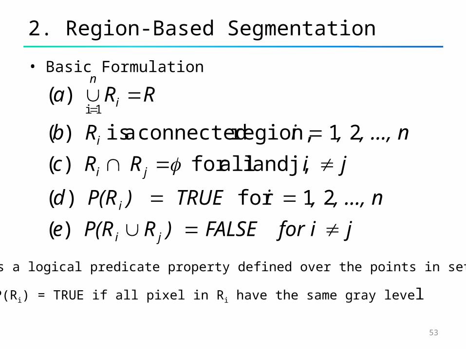
• Basic Formulation

jfor i FALSE) RP(Re

, ..., n, i TRUE) P(Rd

ji RRc

, ..., n, i Rb

RRa

ji

i

ji

i

i

n

)(

21for )(

j, and i allfor )(

21 region, connected a is )(

)(1i

P(Ri) is a logical predicate property defined over the points in set Ri

ex. P(Ri) = TRUE if all pixel in Ri have the same gray level

54

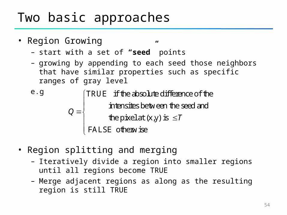
Two basic approaches

• Region Growing– start with a set of “seed” points– growing by appending to each seed those neighbors that have

similar properties such as specific ranges of gray level

e.g

• Region splitting and merging– Iteratively divide a region into smaller regions until all regions

become TRUE– Merge adjacent regions as along as the resulting region is still

TRUE

TRUE if the absolute difference of the

intensites between the seed and

the pixel at (x,y) is

FALSE otherwise

QT

55

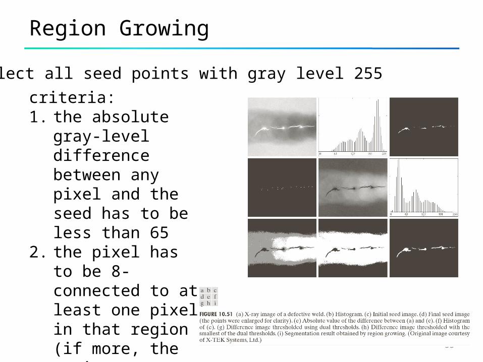
Region Growing

Select all seed points with gray level 255

criteria:1. the absolute gray-

level difference between any pixel and the seed has to be less than 65

2. the pixel has to be 8-connected to at least one pixel in that region (if more, the regions are merged)

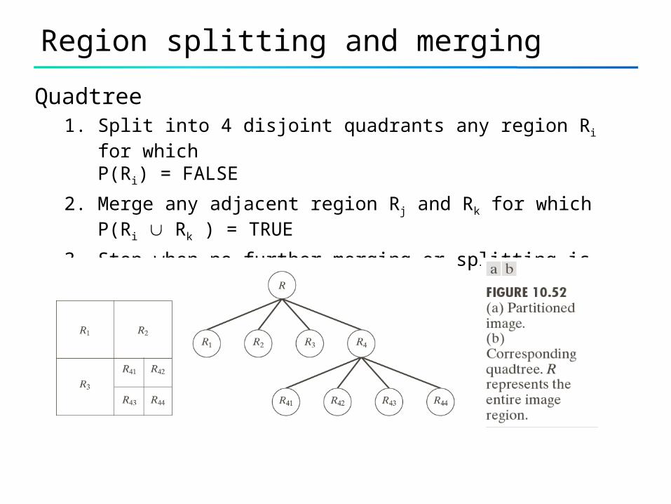
Region splitting and merging

Quadtree1. Split into 4 disjoint quadrants any region Ri for which

P(Ri) = FALSE

2. Merge any adjacent region Rj and Rk for which P(Ri Rk ) = TRUE

3. Stop when no further merging or splitting is possible.

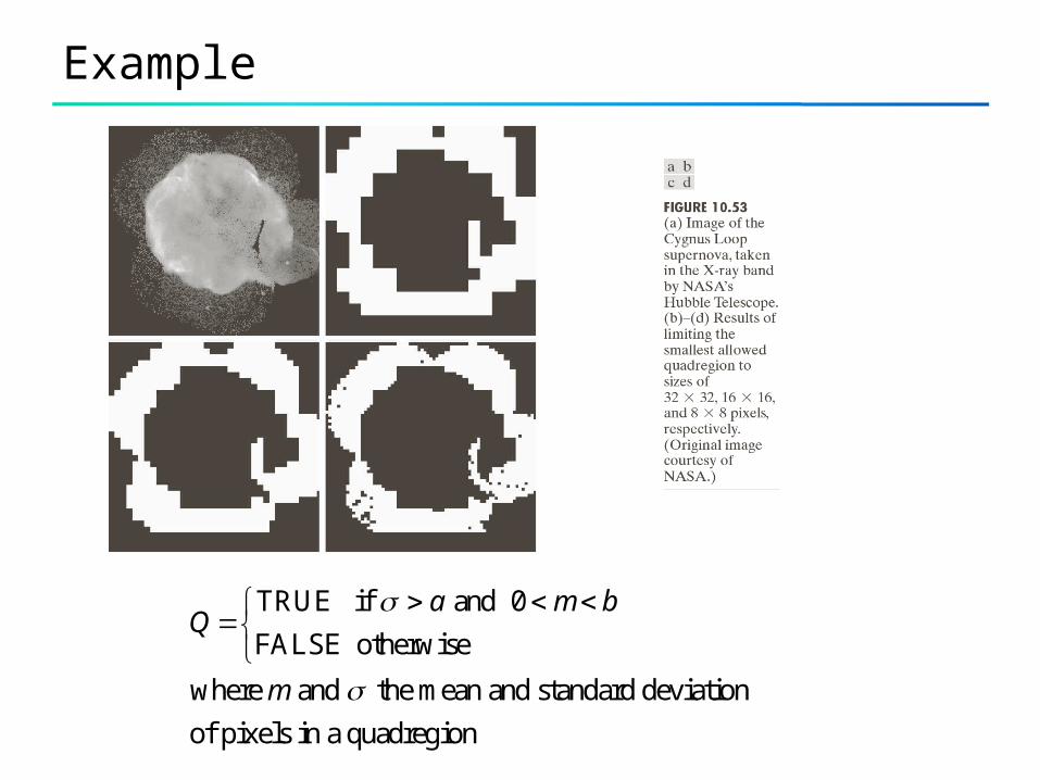
Example

TRUE if and 0

FALSE otherwise

where and the mean and standard deviation

of pixels in a quadregion

a m bQ

m

58

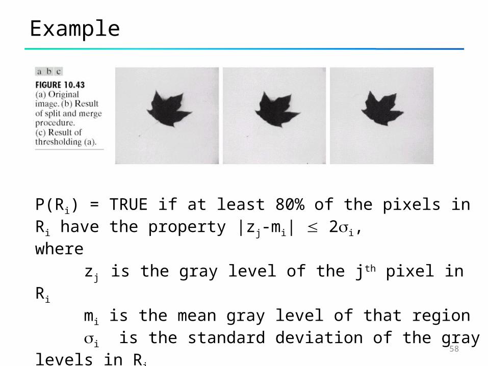
Example

P(Ri) = TRUE if at least 80% of the pixels in Ri have the property |zj-mi| 2i, where

zj is the gray level of the jth pixel in Ri

mi is the mean gray level of that regioni is the standard deviation of the gray levels in Ri

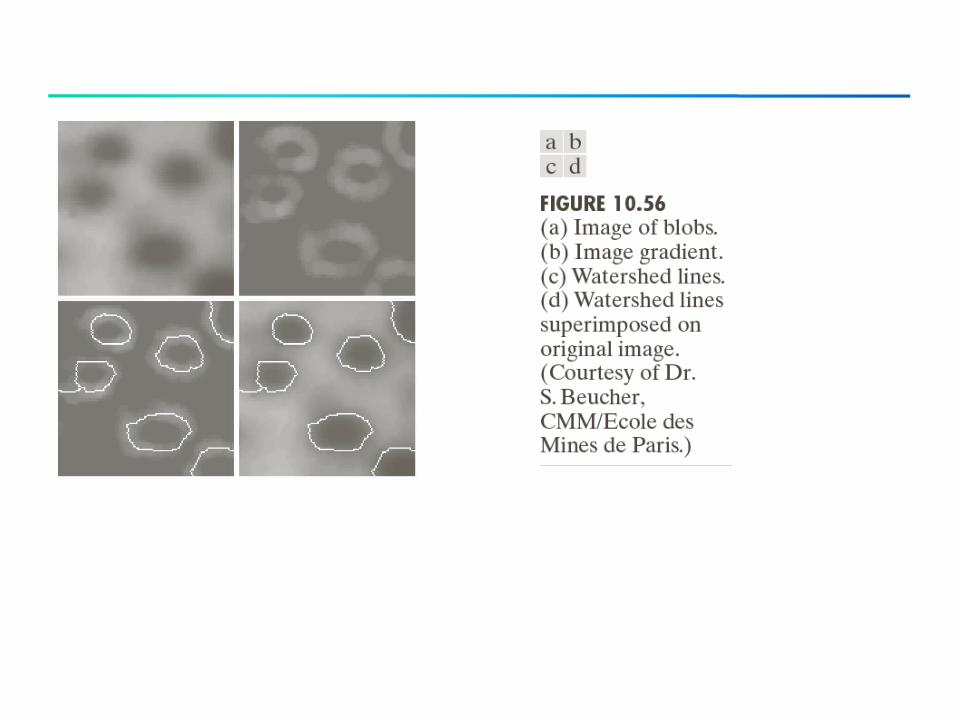
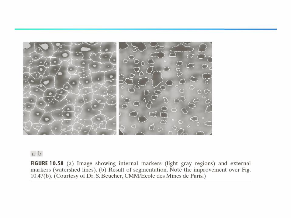
Segmentation using Watersheds

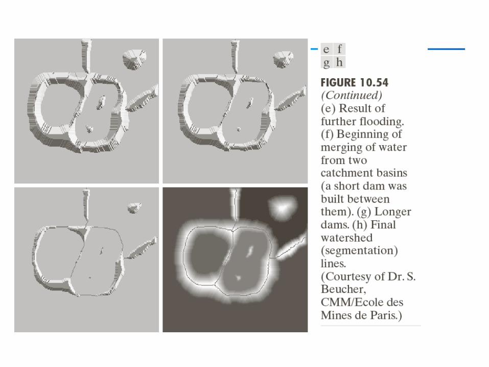
• The concept of watersheds– View an image as 3-D graphics– Three types of points

• Local minimum• Point at which water will flow to a local minimum,

also called catchment basin, or watershed.• Point at which water can equally flow to more than

one local minimum points, also called divide lines, or watershed lines

• Segmentation by watershed lines

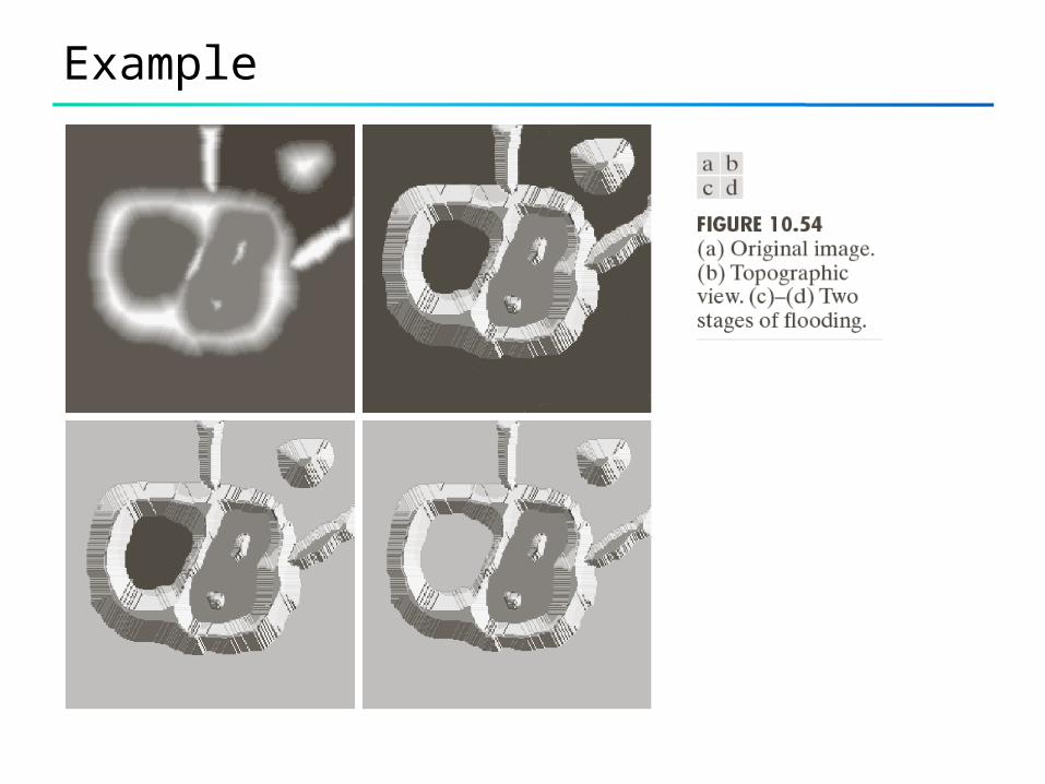
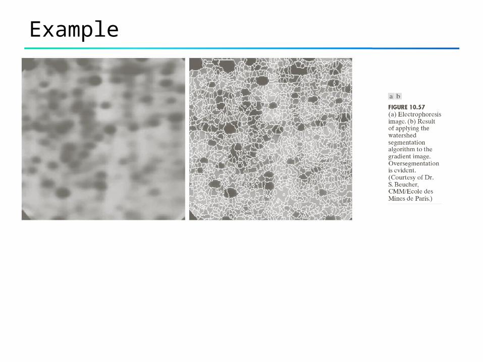
Example

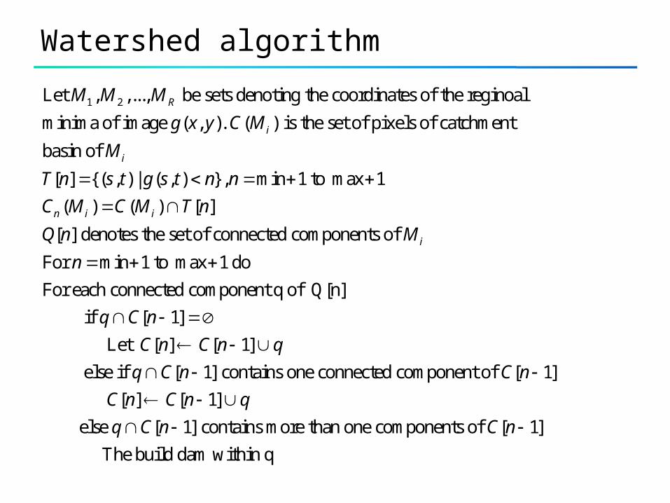
Watershed algorithm

1 2Let , ,..., be sets denoting the coordinates of the reginoal

minima of image ( , ). ( ) is the set of pixels of catchment

basin of

[ ] {( , ) | ( , ) }, min 1 to max 1

( ) ( ) [ ]

[ ]

R

i

i

n i i

M M M

g x y C M

M

T n s t g s t n n

C M C M T n

Q n

denotes the set of connected components of

For min 1 to max 1 do

For each connected component q of Q[n]

if [ 1]

Let [ ] [ 1]

else if [ 1] contains

iM

n

q C n

C n C n q

q C n

one connected component of [ 1]

[ ] [ 1]

else [ 1] contains more than one components of [ 1]

The build dam within q

C n

C n C n q

q C n C n

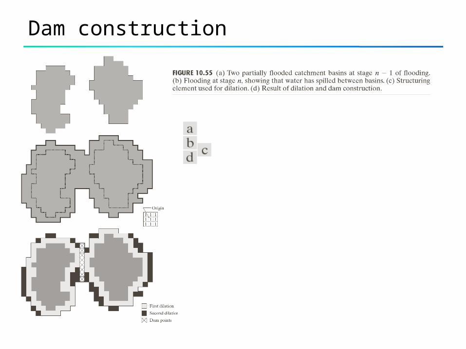
Dam construction

Example