Lecture 15: Object recognition: Bag of Words models Part...

Lecture 15 -Fei-Fei Li

Lecture 15: Object recognition:

Bag of Words models &Part‐based generative models

Professor Fei‐Fei LiStanford Vision Lab

14‐Nov‐111


Basic issues

• Representation– How to represent an object category; which classification scheme?

• Learning– How to learn the classifier, given training data

• Recognition– How the classifier is to be used on novel data

14‐Nov‐112


What we will learn today?

• Bag of Words model (Problem Set 4 (Q2))– Basic representation– Different learning and recognition algorithms

• Constellation model– Weakly supervised training– One‐shot learning (supplementary materials)

• (Problem Set 4 (Q1))

14‐Nov‐113


Part 1: Bag‐of‐words models

This segment is based on the tutorial “Recognizing and Learning Object Categories: Year 2007”, by Prof L. Fei‐Fei, A. Torralba, and R. Fergus

14‐Nov‐114


Related works

• Early “bag of words” models: mostly texture recognition– Cula & Dana, 2001; Leung & Malik 2001; Mori, Belongie & Malik, 2001;

Schmid 2001; Varma & Zisserman, 2002, 2003; Lazebnik, Schmid & Ponce, 2003;

• Hierarchical Bayesian models for documents (pLSA, LDA, etc.)– Hoffman 1999; Blei, Ng & Jordan, 2004; Teh, Jordan, Beal & Blei, 2004

• Object categorization– Csurka, Bray, Dance & Fan, 2004; Sivic, Russell, Efros, Freeman &

Zisserman, 2005; Sudderth, Torralba, Freeman & Willsky, 2005;

• Natural scene categorization– Vogel & Schiele, 2004; Fei‐Fei & Perona, 2005; Bosch, Zisserman &

Munoz, 2006

14‐Nov‐115


Object Bag of ‘words’

14‐Nov‐116


Analogy to documentsOf all the sensory impressions proceeding to the brain, the visual experiences are the dominant ones. Our perception of the world around us is based essentially on the messages that reach the brain from our eyes. For a long time it was thought that the retinal image was transmitted point by point to visual centers in the brain; the cerebral cortex was a movie screen, so to speak, upon which the image in the eye was projected. Through the discoveries of Hubel and Wiesel we now know that behind the origin of the visual perception in the brain there is a considerably more complicated course of events. By following the visual impulses along their path to the various cell layers of the optical cortex, Hubel and Wiesel have been able to demonstrate that the message about the image falling on the retina undergoes a step-wise analysis in a system of nerve cells stored in columns. In this system each cell has its specific function and is responsible for a specific detail in the pattern of the retinal image.

sensory, brain, visual, perception,

retinal, cerebral cortex,eye, cell, optical

nerve, imageHubel, Wiesel

China is forecasting a trade surplus of $90bn (£51bn) to $100bn this year, a threefold increase on 2004's $32bn. The Commerce Ministry said the surplus would be created by a predicted 30% jump in exports to $750bn, compared with a 18% rise in imports to $660bn. The figures are likely to further annoy the US, which has long argued that China's exports are unfairly helped by a deliberately undervalued yuan. Beijing agrees the surplus is too high, but says the yuan is only one factor. Bank of China governor Zhou Xiaochuan said the country also needed to do more to boost domestic demand so more goods stayed within the country. China increased the value of the yuan against the dollar by 2.1% in July and permitted it to trade within a narrow band, but the US wants the yuan to be allowed to trade freely. However, Beijing has made it clear that it will take its time and tread carefully before allowing the yuan to rise further in value.

China, trade, surplus, commerce,

exports, imports, US, yuan, bank, domestic,

foreign, increase, trade, value

14‐Nov‐117


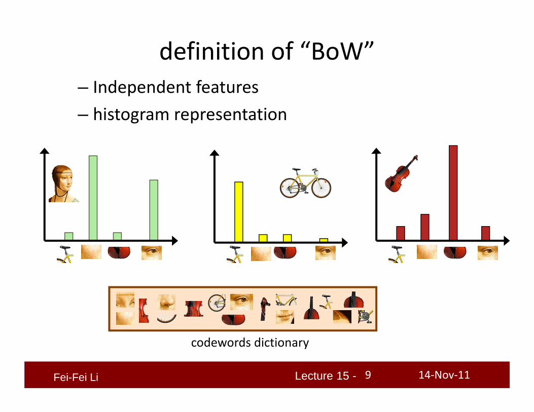
– Independent features

definition of “BoW”

face bike violin

14‐Nov‐118


definition of “BoW”– Independent features – histogram representation

codewords dictionary

14‐Nov‐119


categorydecision

Representation

feature detection& representation


image representation

category models(and/or) classifiers

recognitionle

arni

ng

14‐Nov‐1110


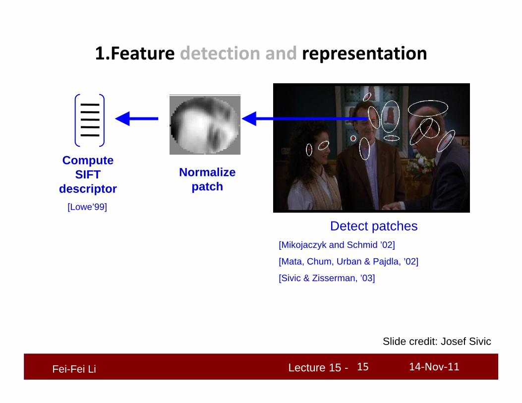
1.Feature detection and representation

14‐Nov‐1111



• Regular grid– Vogel & Schiele, 2003– Fei‐Fei & Perona, 2005

14‐Nov‐1112




• Interest point detector– Csurka, et al. 2004– Fei‐Fei & Perona, 2005– Sivic, et al. 2005

14‐Nov‐1113




• Interest point detector– Csurka, Bray, Dance & Fan, 2004– Fei‐Fei & Perona, 2005– Sivic, Russell, Efros, Freeman & Zisserman, 2005

• Other methods– Random sampling (Vidal‐Naquet & Ullman, 2002)– Segmentation based patches (Barnard, Duygulu, Forsyth, de Freitas, Blei, Jordan, 2003)

14‐Nov‐1114



Normalize patch

Detect patches[Mikojaczyk and Schmid ’02]

[Mata, Chum, Urban & Pajdla, ’02]

[Sivic & Zisserman, ’03]

Compute SIFT

descriptor[Lowe’99]

Slide credit: Josef Sivic

14‐Nov‐1115


…


14‐Nov‐1116


2. Codewords dictionary formation

…

14‐Nov‐1117



Clustering/vector quantization

…

Cluster center= code word

14‐Nov‐1118



Fei-Fei et al. 2005

14‐Nov‐1119


Image patch examples of codewords

Sivic et al. 2005

14‐Nov‐1120


Visual vocabularies: Issues

• How to choose vocabulary size?– Too small: visual words not representative of all patches– Too large: quantization artifacts, overfitting

• Computational efficiency– Vocabulary trees

(Nister & Stewenius, 2006)

14‐Nov‐1121


3. Bag of word representation

Codewords dictionary • Nearest neighbors assignment• K‐D tree search strategy

14‐Nov‐1122


3. Bag of word representation

Codewords dictionary codewords

frequ

ency

….

14‐Nov‐1123


feature detection& representation


image representation

Representation

1.2.

3.

14‐Nov‐1124


categorydecision



Learning and Recognition

14‐Nov‐1125




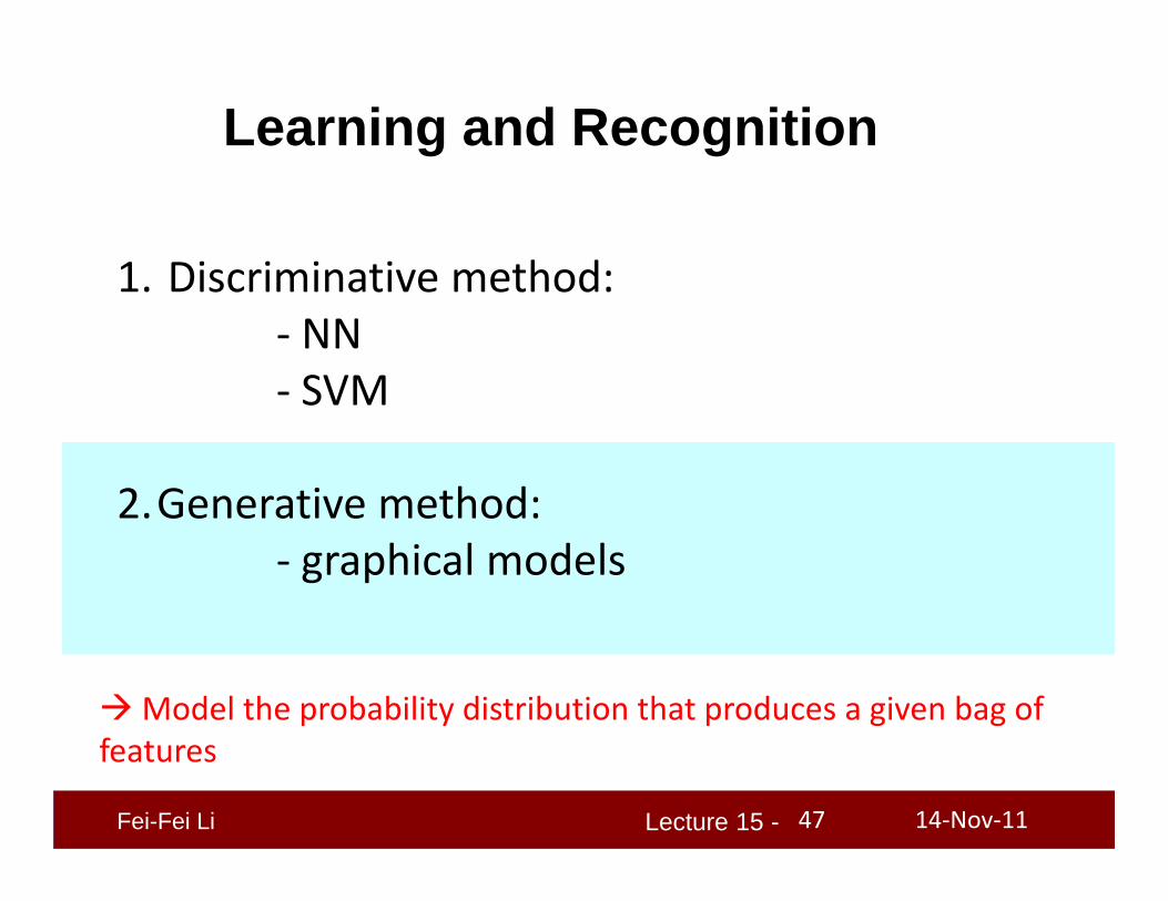
1. Discriminative method: - NN- SVM

2.Generative method: - graphical models

14‐Nov‐1126


category models

Class 1 Class N

… ……

Discriminative classifiers

Model space

14‐Nov‐1127


Discriminative classifiers

Query image

Winning class: pink

Model space

14‐Nov‐1128


Nearest Neighborsclassifier

Query image

Winning class: pink

• Assign label of nearest training data point to each test data point

Model space

14‐Nov‐1129


Query image

• For a new point, find the k closest points from training data• Labels of the k points “vote” to classify• Works well provided there is lots of data and the distance function is good

K- Nearest Neighborsclassifier

Model space

Winning class: pink

14‐Nov‐1130


• For k dimensions: k‐D tree = space‐partitioning data structure for organizing points in a k‐dimensional space• Enable efficient search

from Duda et al.

K- Nearest Neighborsclassifier

• Voronoi partitioning of feature space for 2‐category 2‐D and 3‐D data

• Nice tutorial: http://www.cs.umd.edu/class/spring2002/cmsc420‐0401/pbasic.pdf

14‐Nov‐1131


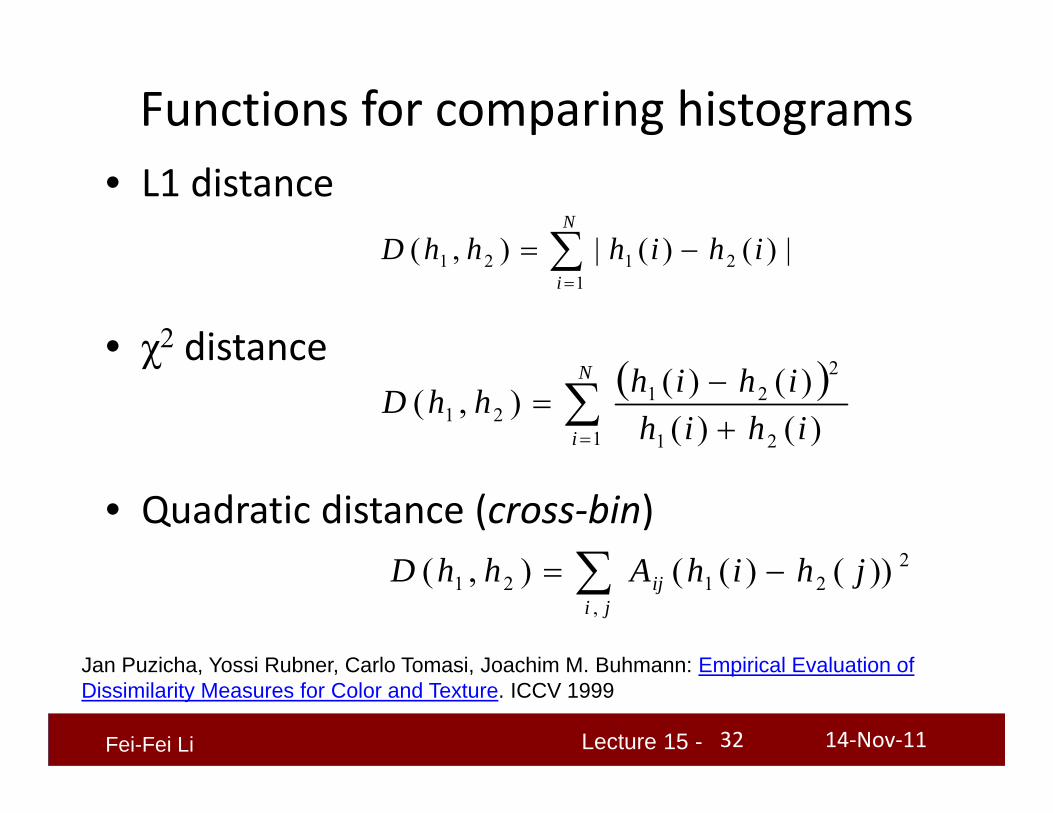
Functions for comparing histograms• L1 distance

• χ2 distance

• Quadratic distance (cross‐bin)

N

iihihhhD

12121 |)()(|),(

Jan Puzicha, Yossi Rubner, Carlo Tomasi, Joachim M. Buhmann: Empirical Evaluation of Dissimilarity Measures for Color and Texture. ICCV 1999

N

i ihihihihhhD

1 21

221

21 )()()()(),(

ji

ij jhihAhhD,

22121 ))()((),(

14‐Nov‐1132



1. Discriminative method: - NN- SVM

2.Generative method: - graphical models

14‐Nov‐1133


Discriminative classifiers(linear classifier)

Model spacecategory models

Class 1 Class N

… ……

14‐Nov‐1134


Support vector machines• Find hyperplane that maximizes the margin between the positive and

negative examples

MarginSupport vectors

Distance between point and hyperplane: ||||

||wwx bi

Support vectors: 1 bi wx

Margin = 2 / ||w||

Credit slide: S. Lazebnik

i iii y xw

bybi iii xxxw

Classification function (decision boundary):

Solution:

14‐Nov‐1135


Support vector machines• Classification

Margin

bybi iii xxxw

2010

classbifclassbif

wxwx

Test point

C. Burges, A Tutorial on Support Vector Machines for Pattern Recognition, Data Mining and Knowledge Discovery, 1998

14‐Nov‐1136


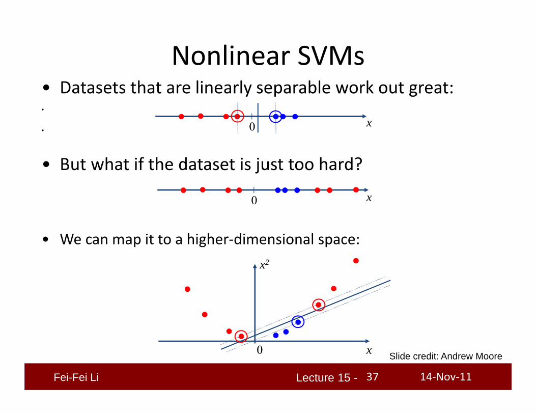
• Datasets that are linearly separable work out great:•

•

• But what if the dataset is just too hard?

• We can map it to a higher‐dimensional space:

0 x

0 x

0 x

x2

Nonlinear SVMs

Slide credit: Andrew Moore

14‐Nov‐1137


Φ: x→ φ(x)

Nonlinear SVMs• General idea: the original input space can always be mapped

to some higher‐dimensional feature space where the training set is separable:

Slide credit: Andrew Moorelifting transformation

14‐Nov‐1138


Nonlinear SVMs• Nonlinear decision boundary in the original feature space:

bKyi

iii ),( xx

C. Burges, A Tutorial on Support Vector Machines for Pattern Recognition, Data Mining and Knowledge Discovery, 1998

•The kernel K = product of the lifting transformation φ(x):

K(xi,xjj) = φ(xi ) · φ(xj)NOTE:• It is not required to compute φ(x) explicitly:• The kernel must satisfy the “Mercer inequality”

14‐Nov‐1139


Kernels for bags of features

• Histogram intersection kernel:

• Generalized Gaussian kernel:

• D can be Euclidean distance, χ2 distance etc…

N

iihihhhI

12121 ))(),(min(),(

2

2121 ),(1exp),( hhDA

hhK

J. Zhang, M. Marszalek, S. Lazebnik, and C. Schmid, Local Features and Kernels for Classifcation of Texture and Object Categories: A Comprehensive Study, IJCV 2007

14‐Nov‐1140


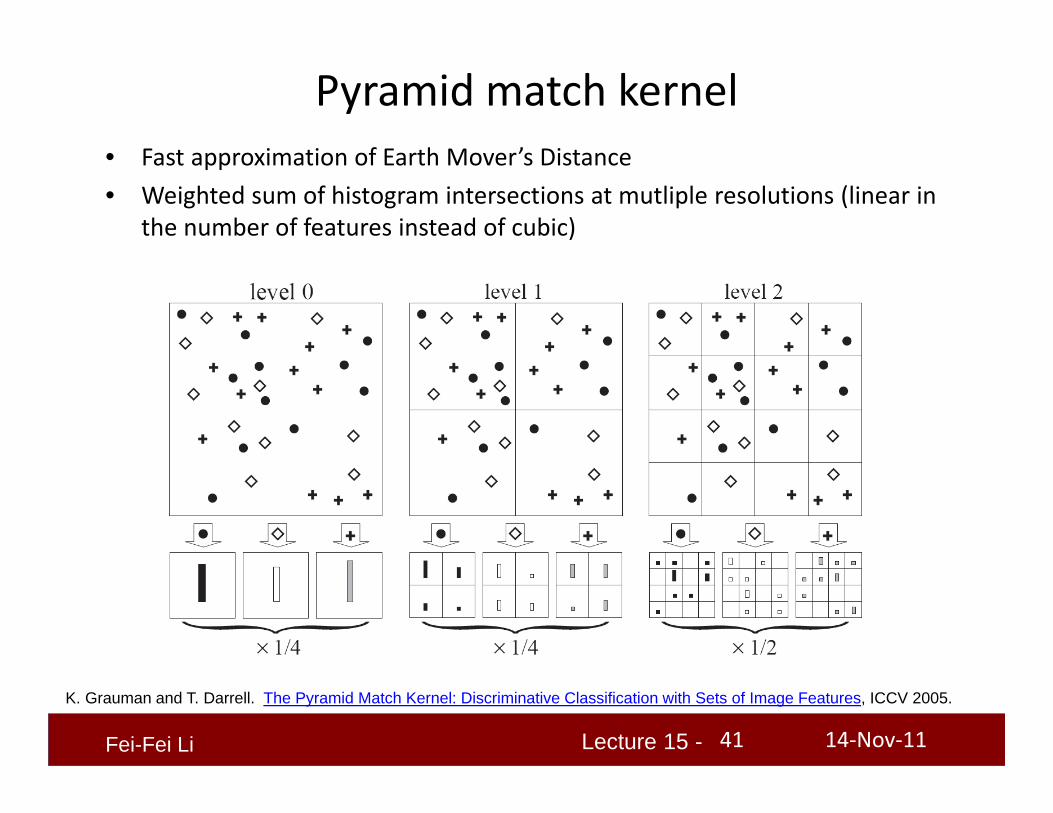
Pyramid match kernel• Fast approximation of Earth Mover’s Distance• Weighted sum of histogram intersections at mutliple resolutions (linear in

the number of features instead of cubic)

K. Grauman and T. Darrell. The Pyramid Match Kernel: Discriminative Classification with Sets of Image Features, ICCV 2005.

14‐Nov‐1141


Spatial Pyramid Matching

Beyond Bags of Features: Spatial Pyramid Matching for Recognizing Natural Scene Categories. S. Lazebnik, C. Schmid, and J. Ponce. CVPR 2006

14‐Nov‐1142


What about multi‐class SVMs?

• No “definitive” multi‐class SVM formulation• In practice, we have to obtain a multi‐class SVM by combining

multiple two‐class SVMs • One vs. others

– Traning: learn an SVM for each class vs. the others– Testing: apply each SVM to test example and assign to it the class of

the SVM that returns the highest decision value

• One vs. one– Training: learn an SVM for each pair of classes– Testing: each learned SVM “votes” for a class to assign to the test

example

Credit slide: S. Lazebnik

14‐Nov‐1143


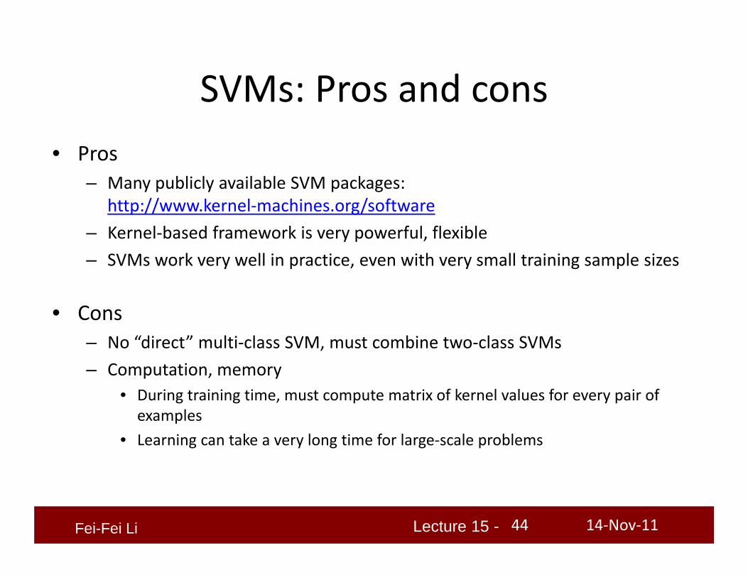
SVMs: Pros and cons• Pros

– Many publicly available SVM packages:http://www.kernel‐machines.org/software

– Kernel‐based framework is very powerful, flexible– SVMs work very well in practice, even with very small training sample sizes

• Cons– No “direct” multi‐class SVM, must combine two‐class SVMs– Computation, memory

• During training time, must compute matrix of kernel values for every pair of examples

• Learning can take a very long time for large‐scale problems

14‐Nov‐1144

Lecture 15 -

Object recognition results

• ETH‐80 database of 8 object classes (Eichhorn and Chapelle 2004)

• Features: – Harris detector– PCA‐SIFT descriptor, d=10

Kernel Complexity Recognition rateMatch [Wallraven et al.] 84%

Bhattacharyya affinity [Kondor & Jebara]

85%

Pyramid match 84%Slide credit: Kristen Grauman

14‐Nov‐11


Discriminative models

Support Vector Machines

Guyon, Vapnik, Heisele, Serre, Poggio…

Boosting

Viola, Jones 2001, Torralba et al. 2004, Opelt et al. 2006,…

106 examples

Nearest neighbor

Shakhnarovich, Viola, Darrell 2003Berg, Berg, Malik 2005...

Neural networks

Source: Vittorio Ferrari, Kristen Grauman, Antonio Torralba

Latent SVMStructural SVM

Felzenszwalb 00Ramanan 03…

LeCun, Bottou, Bengio, Haffner 1998Rowley, Baluja, Kanade 1998…

14‐Nov‐1146



1. Discriminative method: ‐ NN‐ SVM

2.Generative method: ‐ graphical models

Model the probability distribution that produces a given bag of features

14‐Nov‐1147


Generative models

1. Naïve Bayes classifier– Csurka Bray, Dance & Fan, 2004

2. Hierarchical Bayesian text models (pLSA and LDA)

– Background: Hoffman 2001, Blei, Ng & Jordan, 2004– Object categorization: Sivic et al. 2005, Sudderth et al.

2005– Natural scene categorization: Fei‐Fei et al. 2005

14‐Nov‐1148


• w: a collection of all N codewords in the imagew = [w1,w2,…,wN]

• c: category of the image

Some notations

14‐Nov‐1149

Lecture 15 -

wN

c

the Naïve Bayes model

)|()( cwpcp)|( wcp

14‐Nov‐11

Prior prob. of the object classes

Image likelihoodgiven the class

Graphical model

Posterior =probability that image I is of category c

Lecture 15 -

wN

c

the Naïve Bayes model

)|()( cwpcp

N

nn cwpcp

1

)|()(

Object classdecision

)|( wcpc

c maxarg

Likelihood of ith visual wordgiven the class

Estimated by empirical frequencies of code words in images from a given class

14‐Nov‐11

Graphical model


Csurka et al. 2004

14‐Nov‐1152


Csurka et al. 2004

14‐Nov‐1153


Other generative BoWmodels

• Hierarchical Bayesian topic models (e.g. pLSAand LDA)

– Object categorization: Sivic et al. 2005, Sudderth et al. 2005– Natural scene categorization: Fei‐Fei et al. 2005

14‐Nov‐1154


Generative vs discriminative

• Discriminative methods– Computationally efficient & fast

• Generative models– Convenient for weakly‐ or un‐supervised, incremental training

– Prior information– Flexibility in modeling parameters

14‐Nov‐1155


• No rigorous geometric information of the object components

• It’s intuitive to most of us that objects are made of parts – no such information

• Not extensively tested yet for– View point invariance– Scale invariance

• Segmentation and localization unclear

Weakness of BoW the models

14‐Nov‐1156


What we will learn today?




14‐Nov‐1157


Model: Parts and Structure

14‐Nov‐1158


• Fischler & Elschlager 1973

• Yuille ‘91• Brunelli & Poggio ‘93• Lades, v.d. Malsburg et al. ‘93• Cootes, Lanitis, Taylor et al. ‘95• Amit & Geman ‘95, ‘99 • et al. Perona ‘95, ‘96, ’98, ’00, ‘03• Huttenlocher et al. ’00• Agarwal & Roth ’02

etc…

Parts and Structure Literature

14‐Nov‐1159


The Constellation ModelT. Leung

M. Burl

Representation

Detection

Shape statistics – F&G ’95Affine invariant shape – CVPR ‘98

CVPR ‘96ECCV ‘98

M. WeberM. Welling Unsupervised Learning

ECCV ‘00Multiple views - F&G ’00 Discovering categories - CVPR ’00

R. Fergus

L. Fei-Fei

Joint shape & appearance learningGeneric feature detectors

One-Shot LearningIncremental learning

CVPR ’03Polluted datasets - ECCV ‘04

ICCV ’03CVPR ‘04

14‐Nov‐1160


A B

DC

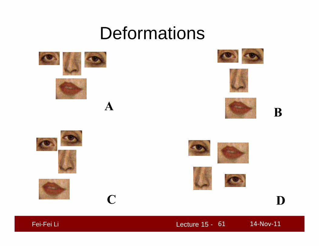
Deformations

14‐Nov‐1161


Presence / Absence of Features

occlusion

14‐Nov‐1162


Background clutter

14‐Nov‐1163


Foreground modelGenerative probabilistic model

Gaussian shape pdfClutter modelUniform shape pdfProb. of detection

0.8 0.75

0.9

# detections

pPoisson(N2|2)

pPoisson(N1|1)

pPoisson(N3|3)

Assumptions: (a) Clutter independent of foreground detections(b) Clutter detections independent of each other

Example1. Object Part Positions

3a. N false detect2. Part Absence

N1

N2

3b. Position f. detect

N3

14‐Nov‐1164


Learning Models `Manually’

• Obtain set of training images

• Label parts by hand, train detectors

• Learn model from labeled parts

• Choose parts

14‐Nov‐1165


Recognition1. Run part detectors exhaustively over image

2032

e.g.

0000

4

3

2

1

h

NNNN

h

1

2

3

3

2

41

1

2 3

1

2

2. Try different combinations of detections in model- Allow detections to be missing (occlusion)

3. Pick hypothesis which maximizes:

4. If ratio is above threshold then, instance detected

),|(),|(

HypClutterDatapHypObjectDatap

14‐Nov‐1166


So far…..• Representation

– Joint model of part locations– Ability to deal with background clutter and occlusions

• Learning– Manual construction of part detectors– Estimate parameters of shape density

• Recognition– Run part detectors over image– Try combinations of features in model– Use efficient search techniques to make fast

14‐Nov‐1167


Unsupervised LearningWeber & Welling et. al.

14‐Nov‐1168


(Semi) Unsupervised learning

•Know if image contains object or not•But no segmentation of object or manual selection of features

14‐Nov‐1169


Unsupervised detector training - 1

• Highly textured neighborhoods are selected automatically• produces 100-1000 patterns per image

10

10

14‐Nov‐1170



“Pattern Space” (100+ dimensions)

14‐Nov‐1171



100-1000 images ~100 detectors

14‐Nov‐1172


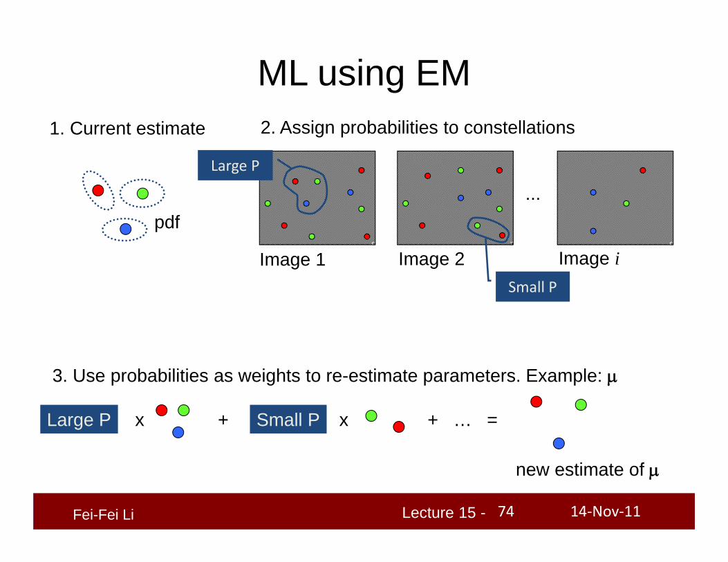
• Task: Estimation of model parameters

Learning

• Let the assignments be a hidden variable and use EM algorithm to learn them and the model parameters

• Chicken and Egg type problem, since we initially know neither:

- Model parameters

- Assignment of regions to foreground / background

• Take training images. Pick set of detectors. Apply detectors.

14‐Nov‐1173


ML using EM1. Current estimate

...

Image 1 Image 2 Image i

2. Assign probabilities to constellations

Large P

Small P

3. Use probabilities as weights to re-estimate parameters. Example:

Large P x + Small P x

pdf

new estimate of

+ … =

14‐Nov‐1174


Detector Selection

ParameterEstimation

Choice 1

Choice 2 ParameterEstimation

Model 1

Model 2

Predict / measure model performance(validation set or directly from model)

Detectors (100)

•Try out different combinations of detectors (Greedy search)

14‐Nov‐1175


Frontal Views of Faces

• 200 Images (100 training, 100 testing)

• 30 people, different for training and testing

14‐Nov‐1176


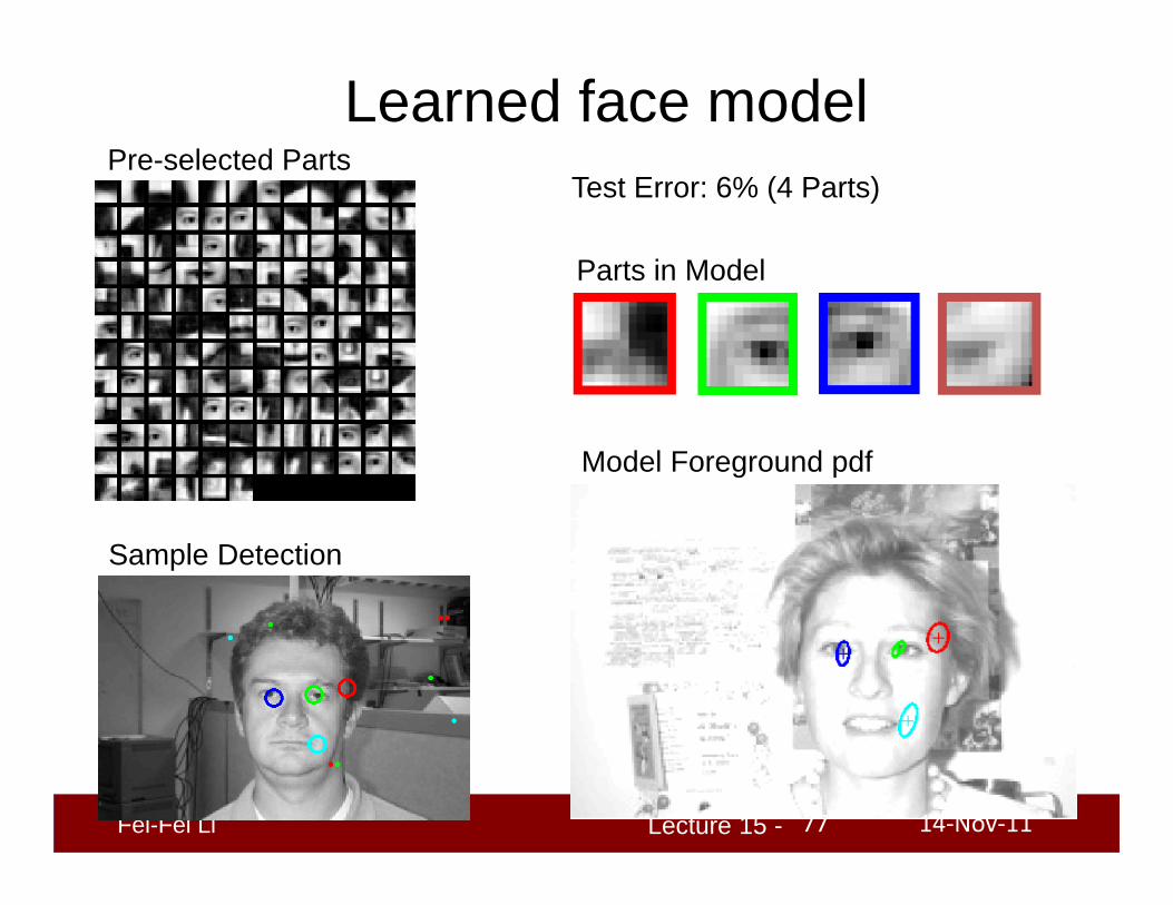
Learned face modelPre-selected Parts

Model Foreground pdf

Sample Detection

Parts in Model

Test Error: 6% (4 Parts)

14‐Nov‐1177


Face images

14‐Nov‐1178


Background images

14‐Nov‐1179


Preselected Parts

Model Foreground pdf

Sample Detection

Parts in Model

Car from RearTest Error: 13% (5 Parts)

14‐Nov‐1180


Detections of Cars

14‐Nov‐1181


Background Images

14‐Nov‐1182


3D Object recognition – Multiple mixture components

14‐Nov‐1183


3D Orientation Tuning

Frontal Profile

0 20 40 60 80 10050

55

60

65

70

75

80

85

90

95

100Orientation Tuning

angle in degrees

% Correct

% Correct

14‐Nov‐1184


So far (2)…..• Representation

– Multiple mixture components for different viewpoints

• Learning– Now semi-unsupervised– Automatic construction and selection of part detectors– Estimation of parameters using EM

• Recognition– As before

• Issues:-Learning is slow (many combinations of detectors)-Appearance learnt first, then shape

14‐Nov‐1185


Issues• Speed of learning

– Slow (many combinations of detectors)• Appearance learnt first, then shape

– Difficult to learn part that has stable location but variable appearance

– Each detector is used as a cross-correlation filter, giving a hard definition of the part’s appearance

• Would like a fully probabilistic representation of the object

14‐Nov‐1186


Object categorization

Fergus et. al.

CVPR ’03, IJCV ‘0614‐Nov‐1187


Detection & Representation of regions

Appearance

Location

Scale

(x,y) coords. of region centre

Radius of region (pixels)

11x11 patchNormalizeProjection onto

PCA basis

c1

c2

c15

……

…..

Gives representation of appearance in low-dimensional vector space

• Find regions within image

• Use salient region operator(Kadir & Brady 01)

14‐Nov‐1188


Motorbikes example•Kadir & Brady saliency region detector

14‐Nov‐1189


Foreground modelGaussian shape pdf

Poission pdf on # detections

Uniform shape pdf

Generative probabilistic model (2)

Clutter model

Gaussian part appearance pdf

Gaussian background appearance pdf

Prob. of detection

0.8 0.75 0.9

Gaussian relative scale pdf

log(scale)

Uniformrelative scale pdf

log(scale)

based on Burl, Weber et al. [ECCV ’98, ’00]

14‐Nov‐1190


MotorbikesSamples from appearance model

14‐Nov‐1191


Recognized Motorbikes

14‐Nov‐1192


Background images evaluated with motorbike model

14‐Nov‐1193


Frontal faces

14‐Nov‐1194


Airplanes

14‐Nov‐1195


Spotted cats

14‐Nov‐1196


Summary of results

Dataset Fixed scale experiment

Scale invariant experiment

Motorbikes 7.5 6.7

Faces 4.6 4.6

Airplanes 9.8 7.0

Cars (Rear) 15.2 9.7

Spotted cats 10.0 10.0

% equal error rateNote: Within each series, same settings used for all datasets

14‐Nov‐1197


Comparison to other methods

Dataset Ours Others

Motorbikes 7.5 16.0 Weber et al. [ECCV ‘00]

Faces 4.6 6.0 Weber

Airplanes 9.8 32.0 Weber

Cars (Side) 11.5 21.0Agarwal

Roth [ECCV ’02]

% equal error rate

14‐Nov‐1198


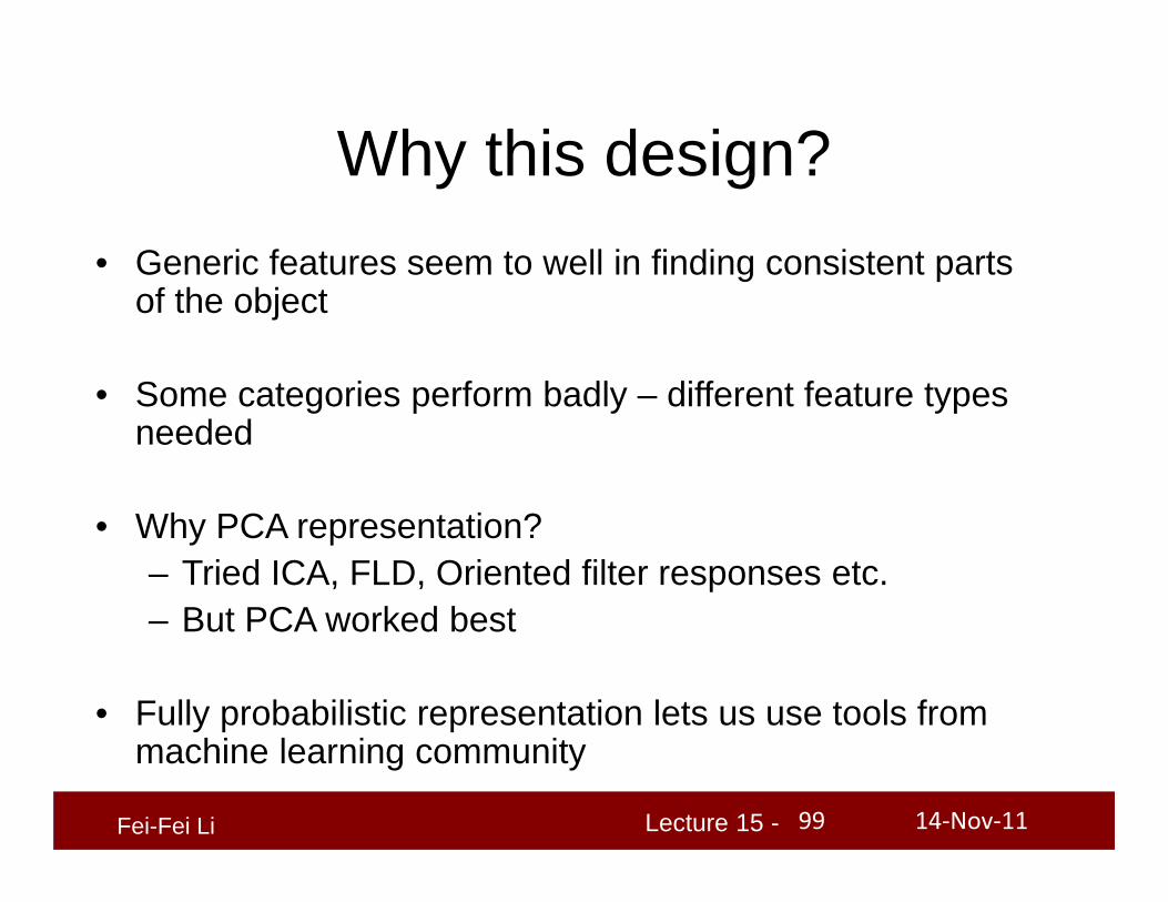
Why this design?• Generic features seem to well in finding consistent parts

of the object

• Some categories perform badly – different feature types needed

• Why PCA representation?– Tried ICA, FLD, Oriented filter responses etc.– But PCA worked best

• Fully probabilistic representation lets us use tools from machine learning community

14‐Nov‐1199


What we have learned today?

14‐Nov‐11100





Supplementary materials

• One‐Shot learning using Constellation Model

14‐Nov‐11101


S. Savarese, 2003

14‐Nov‐11102

Lecture 15 -Fei-Fei Li P. Buegel, 156214‐Nov‐11103


One-Shot learningFei-Fei et. al.

ICCV ’03, PAMI ‘0614‐Nov‐11104


Algorithm Training Examples Categories

Burl, et al. Weber, et al. Fergus, et al. 200 ~ 400

Faces, Motorbikes, Spotted cats, Airplanes,

Cars

Viola et al. ~10,000 Faces

Schneiderman, et al. ~2,000 Faces, Cars

Rowley et al.

~500 Faces

14‐Nov‐11105


1 2 3 4 5 6 7 8 90

10

20

30

40

50

60

log2 (Training images)

Cla

ssifi

catio

n er

ror

(%)

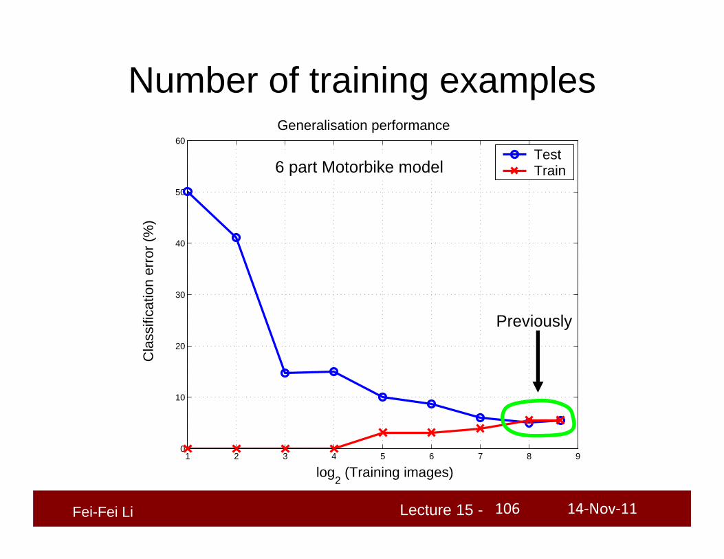
Generalisation performance

TestTrain

Number of training examples

Previously

6 part Motorbike model

14‐Nov‐11106


How do we do better than what statisticians have told us?

• Intuition 1: use Prior information

• Intuition 2: make best use of training information

14‐Nov‐11107


Prior knowledge: meansShapeAppearance

14‐Nov‐11108


MLPrevious Work:



Bayes Rule



14‐Nov‐11110


One-Shot learning: pp object,train



Bayes Rule



14‐Nov‐11111


1

2n

model () space

Each object model

Gaussian shape pdfGaussian part

appearance pdf

Model Structure

14‐Nov‐11112


2n

model distribution: p()• conjugate distribution of p(train|,object)

1

model () space

Each object model

Gaussian shape pdfGaussian part

appearance pdf

Model Structure

14‐Nov‐11113


Learning Model Distribution

• use Prior information

• Bayesian learning

• marginalize over theta

Variational EM (Attias, Hinton, Minka, etc.)

ppp object ,train trainobject,

14‐Nov‐11114


E-Step

Random initializationVariational EM

prior knowledge of p()

new estimate of p(|train)

M-Step

new ’s

14‐Nov‐11115


ExperimentsTraining:

1- 6 randomly

drawn images

Testing:

50 fg/ 50 bg images

object present/absent

Datasets

spotted catsairplanes motorbikesfaces

14‐Nov‐11116


Faces

Airplanes

Motorbikes

Spotted cats

14‐Nov‐11117


Experiments: obtaining priors

spotted cats

airplanes

motorbikes

faces

model () space

14‐Nov‐11118


Experiments: obtaining priors

spotted cats

faces

airplanes

motorbikes

model () space

14‐Nov‐11119



14‐Nov‐11120



14‐Nov‐11121



14‐Nov‐11122



14‐Nov‐11123


Algorithm Training Examples Categories Results(e

rror)

Burl, et al. Weber, et al. Fergus, et al. 200 ~ 400

Faces, Motorbikes, Spotted cats, Airplanes,

Cars

5.6 - 10 %

Viola et al. ~10,000 Faces 7-21%

Schneiderman, et al. ~2,000 Faces, Cars 5.6 – 17%

Rowley et al.

~500 Faces 7.5 –24.1%

BayesianOne-Shot 1 ~ 5 Faces, Motorbikes,

Spotted cats, Airplanes8 –

15 %

14‐Nov‐11124

Lecture 15: Object recognition: Bag of Words models Part...

Documents

Transcript of Lecture 15: Object recognition: Bag of Words models Part...