Lecture 15

Fourier Transforms (cont’d)

Here we list some of the more important properties of Fourier transforms. You have probably seen

many of these, so not all proofs will not be presented. (That being said, most proofs are quite straight-

forward and you are encouraged to try them.) You may find derivations of all of these properties in

the book by Boggess and Narcowich, Section 2.2, starting on p. 98.

Let us first recall the definitions of the Fourier transform (FT) and inverse FT (IFT) that will be

used in this course. Given a function f(t), its Fourier transform F (ω) is defined as

F (ω) =1√2π

∫

∞

−∞

f(t)e−iωtdt. (1)

And given a Fourier transform F (ω), its inverse FT is given by

f(t) =1√2π

∫

∞

−∞

F (ω)eiωtdω. (2)

In what follows, we assume that the functions f(t) and g(t) are differentiable as often as necessary,

and that all necessary integrals exist. (This implies that f(t) → 0 as |t| → ∞.) Regarding notation:

f (n)(t) denotes the nth derivative of f w.r.t. t; F (n)(ω) denotes the nth derivative of F w.r.t. ω.

1. Linearity of the FT operator and the inverse FT operator:

F(f + g) = F(f) + F(g)

F(cf) = c F(f), c ∈ C (or R), (3)

F−1(f + g) = F−1(f) + F−1(g)

F−1(cf) = c F−1(f), c ∈ C (or R), (4)

These follow naturally from the integral definition of the FT.

2. Fourier transform of a product of f with tn:

F(tnf(t)) = inF (n)(ω). (5)

We consider the case n = 1 by taking the derivative of F (ω) in Eq. (1):

F ′(ω) =d

dω

[

1√2π

∫

∞

−∞

f(t)e−iωtdt

]

174

=1√2π

∫

∞

−∞

f(t)d

dω

[

e−iωt]

dt (Leibniz Rule)

=1√2π

∫

∞

−∞

f(t)(−it)e−iωtdt

= −i1√2π

∫

∞

−∞

tf(t)e−iωtdt

= −iF(tf(t)). (6)

Repeated applications of the differentiation operator produces the result,

F (n)(ω) = (−i)nF(tnf(t)), (7)

from which the desired property follows.

3. Inverse Fourier transform of a product of F with ωn:

F−1(ωnF (ω)) = (−i)nf (n)(t). (8)

Here, we start with the definition of the inverse FT in Eq. (2) and differentiate both sides

repeatedly with respect to t. The reader will note a kind of reciprocity between this result and

the previous one.

4. Fourier transform of an nth derivative:

F(f (n)(t)) = (iω)nF (ω). (9)

This is a consequence of 3. above.

5. Inverse Fourier transform of an nth derivative:

F−1(F (n)(ω)) = (−it)nf(t). (10)

This is a consequence of 2. above.

6. Fourier transform of a translation (“Spatial- or Temporal-shift Theorem”):

F(f(t − a)) = e−iωaF (ω). (11)

Because this result is very important, we provide a proof, even though it is very simple:

F(f(t − a)) =1√2π

∫

∞

−∞

f(t − a)e−iωtdt

175

=1√2π

∫

∞

−∞

f(s)e−iω(s+a)ds (s = t − a, dt = ds, etc.)

= e−iωa 1√2π

∫

∞

−∞

f(s)e−iωsds

= e−iωaF (ω). (12)

7. Fourier transform of a “modulation” (“Frequency-shift Theorem”:

F(eiω0tf(t)) = F (ω − ω0). (13)

The proof is very simple:

F(eiω0tf(t)) =1√2π

∫

∞

−∞

eiω0tf(t)e−iωtdt

=1√2π

∫

∞

−∞

f(t)e−i(ω−ω0)tdt

= F (ω − ω0). (14)

We’ll return to this important result to discuss it in more detail.

8. Fourier transform of a scaled function (“Scaling Theorem”): For a b > 0,

F(f(bt)) =1

bF

(ω

b

)

. (15)

Once again, because of its importance, we provide a proof, which is also quite simple:

F(f(bt)) =1√2π

∫

∞

−∞

f(bt)e−iωtdt

=1

b

1√2π

∫

∞

−∞

f(s)e−iωs/bds (s = bt, dt =1

bds, etc.)

=1

b

1√2π

∫

∞

−∞

f(s)e−i(ωb )sds

=1

bF

(ω

b

)

. (16)

We’ll also return to this result to discuss it in more detail.

9. Convolution Theorem: We denote the convolution of two functions f and g as “f ∗g,” defined

as follows:

(f ∗ g)(t) =

∫

∞

−∞

f(t − s)g(s) ds

=

∫

∞

−∞

f(s)g(t − s) ds. (17)

176

This is a continuous version of the convolution operation introduced for the discrete Fourier

transform. In special cases, it may be viewed as a local averaging procedure, as we’ll show

below.

Theorem: If h(t) = (f ∗ g)(t), then the FT of H is given by

H(ω) =√

2πF (ω)G(ω). (18)

Another way of writing this is

F(f ∗ g) =√

2πFG. (19)

By taking inverse FTs of both sides and moving the factor√

2π,

F−1(FG) =1√2π

f ∗ g. (20)

Proof: By definition, the Fourier transform of h is given by

H(ω) =1√2π

∫

∞

−∞

∫

∞

−∞

f(t − s)g(s) ds e−iωt dt

=1√2π

∫

∞

−∞

∫

∞

−∞

f(t − s)g(s) ds e−iω(t−s)e−iωs dt. (21)

Noting the appearance of t−s and s in the exponentials and in the functions f and g, respectively,

we make the following change of variables,

u(s, t) = s, v(s, t) = t − s. (22)

The Jacobian of this transformation is

J =

∣

∣

∣

∣

∣

∣

∂u/∂s ∂u/∂t

∂v/∂s ∂v/∂t

∣

∣

∣

∣

∣

∣

=

∣

∣

∣

∣

∣

∣

1 0

−1 1

∣

∣

∣

∣

∣

∣

= 1. (23)

Therefore, we have ds dt = du dv. Furthermore, the above double integral is separable and may

be written as

H(ω) =1√2π

(∫

∞

−∞

f(v)e−iωv dv

) (∫

∞

−∞

f(u)e−iωu du

)

=√

2π1√2π

(∫

∞

−∞

f(v)e−iωv dv

)

1√2π

(∫

∞

−∞

f(u)e−iωu du

)

=√

2π F (ω)G(ω), (24)

which completes the derivation.

177

A more detailed look at some properties of Fourier transforms

The “Frequency-shift Theorem”

There are two interesting consequences of the Frequency-shift Theorem,

F(eiω0tf(t)) = F (ω − ω0). (25)

We may be interested in computing the FT of the product of either cos ω0t or sin ω0t with a

function f(t), which are known as (amplitude) modulations of f(t). In this case, we express

these trigonometric functions in terms of appropriate complex exponentials and then employ the

above Shift Theorem.

First of all, we start with the relations

cos ω0t =1

2

[

eω0t + e−ω0t]

sin ω0t =1

2i

[

eω0t − e−ω0t]

. (26)

From these results and the Frequency Shift Theorem, we have

F(cos ω0tf(t)) =1

2[F (ω − ω0) + F (ω + ω0)]

F(sin ω0tf(t)) =1

2i[F (ω − ω0) − F (ω + ω0)] , (27)

where F (ω) denotes the FT of f(t).

To show how these results may be helpful in the computation of FTs, let us revisit Example 2

on Page 6, namely the computation of the FT of the function f(t) defined as the function cos 3t,

but restricted to the interval [−π, π]. We may view f(t) as a product of two functions, i.e.,

f(t) = cos 3t · b(t), (28)

where b(t) denotes the boxcar function of Example 1. From the Frequency Shift Theorem,

F (ω) = F(f(t)) =1

2[B(ω − 3) + B(ω + 3)] , (29)

where

B(ω) =√

2π sinc(πω) =√

2πsin(πω)

πω=

√

2

π

sin(πω)

ω(30)

178

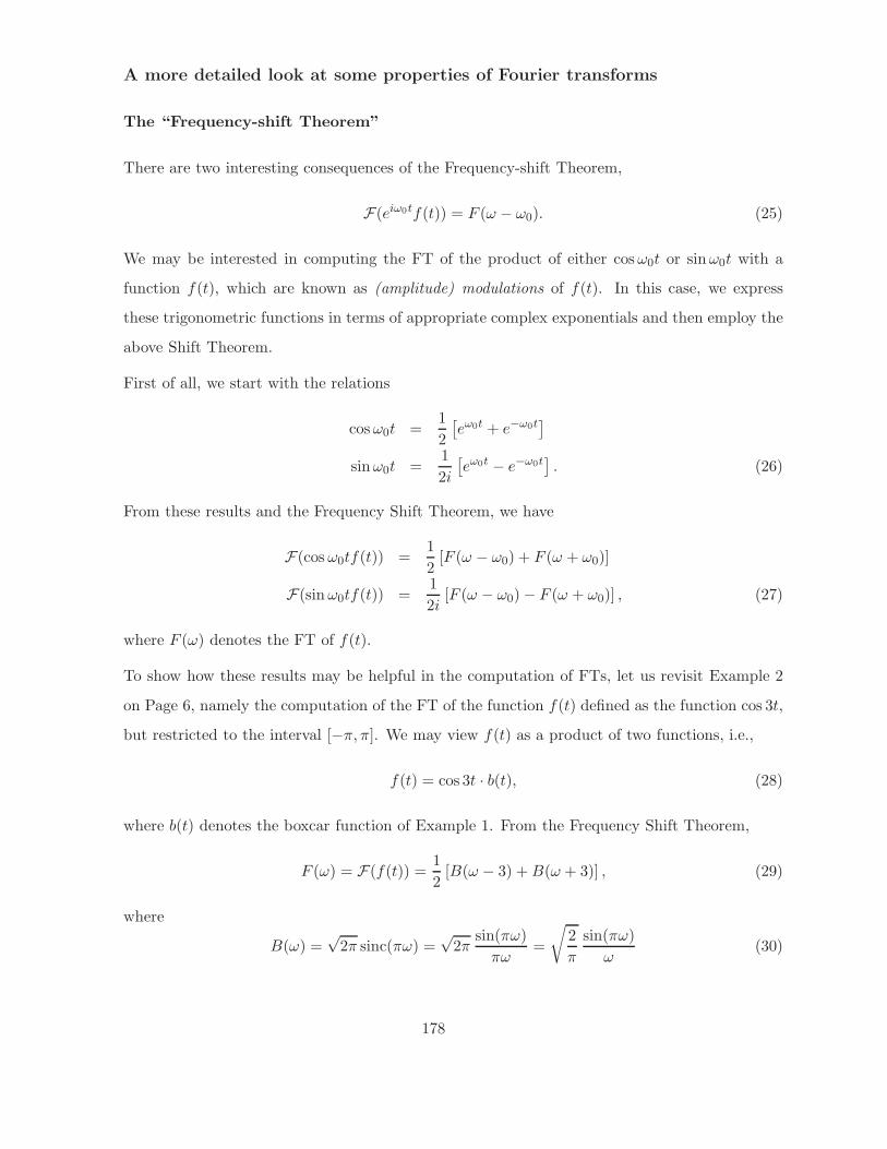
is the FT of the boxcar function b(t). Substitution into the preceeding equation yields

F (ω) =1√2π

[

sin(π(ω − 3))

ω − 3− sin(π(ω + 3))

ω + 3

]

=1√2π

(−2ω)sin(πω)

ω2 − 9

=

√

2

π

ω sin(πω)

9 − ω2, (31)

in agreement with the result obtained for Example 2 earlier.

That being said, it is probably easier now to understand the plot of the Fourier transform that

was presented with Example 2. Instead of trying to decipher the structure of the plot of the

function sin(πω) divided by the polynomial 9 − ω2, one can more easily visualize a sum of two

shifted sinc functions.

The “Scaling Theorem”

Let’s try to get a picture of the Scaling Theorem:

F(f(bt)) =1

bF

(ω

b

)

. (32)

Suppose that b > 1. Then the graph of the function g(t) = f(bt) is obtained from the graph of

f(t) by contracting the latter horizontally toward the y-axis by a factor of 1/b, as sketched in

the plots below.

t2/b

A A

y

t t

y

y = f(t) y = f(bt)

t1 t2 t1/b

Left: Graph of f(t), with two points t1 and t2, where f(t) = A. Right: Graph of f(bt) for b > 1. The two

points at which f(t) = A have now been contracted toward the origin and are at t1/b and t2/b, respectively.

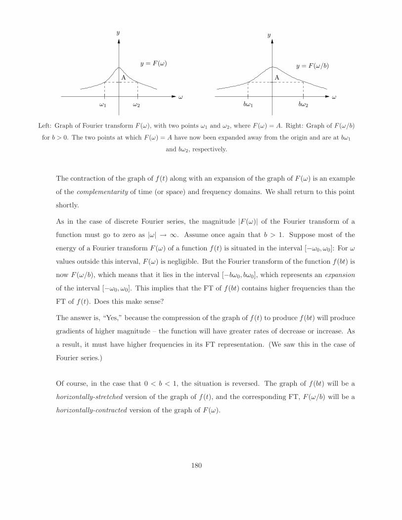
On the other hand, the graph G(ω) = F(

ωb

)

is obtained from the graph of F (ω) by stretching

it outward away by a factor of b from the y-axis, as sketched in the next set of plots below.

179

ω

A

y y

A

y = F (ω) y = F (ω/b)

ω1 ω2 bω1 bω2

ω

Left: Graph of Fourier transform F (ω), with two points ω1 and ω2, where F (ω) = A. Right: Graph of F (ω/b)

for b > 0. The two points at which F (ω) = A have now been expanded away from the origin and are at bω1

and bω2, respectively.

The contraction of the graph of f(t) along with an expansion of the graph of F (ω) is an example

of the complementarity of time (or space) and frequency domains. We shall return to this point

shortly.

As in the case of discrete Fourier series, the magnitude |F (ω)| of the Fourier transform of a

function must go to zero as |ω| → ∞. Assume once again that b > 1. Suppose most of the

energy of a Fourier transform F (ω) of a function f(t) is situated in the interval [−ω0, ω0]: For ω

values outside this interval, F (ω) is negligible. But the Fourier transform of the function f(bt) is

now F (ω/b), which means that it lies in the interval [−bω0, bω0], which represents an expansion

of the interval [−ω0, ω0]. This implies that the FT of f(bt) contains higher frequencies than the

FT of f(t). Does this make sense?

The answer is, “Yes,” because the compression of the graph of f(t) to produce f(bt) will produce

gradients of higher magnitude – the function will have greater rates of decrease or increase. As

a result, it must have higher frequencies in its FT representation. (We saw this in the case of

Fourier series.)

Of course, in the case that 0 < b < 1, the situation is reversed. The graph of f(bt) will be a

horizontally-stretched version of the graph of f(t), and the corresponding FT, F (ω/b) will be a

horizontally-contracted version of the graph of F (ω).

180

The Convolution Theorem

The Convolution Theorem, Eq. (17), is extremely important in signal/image processing, as we

shall see shortly. Let us return to the idea that a convolution may represent a local averaging

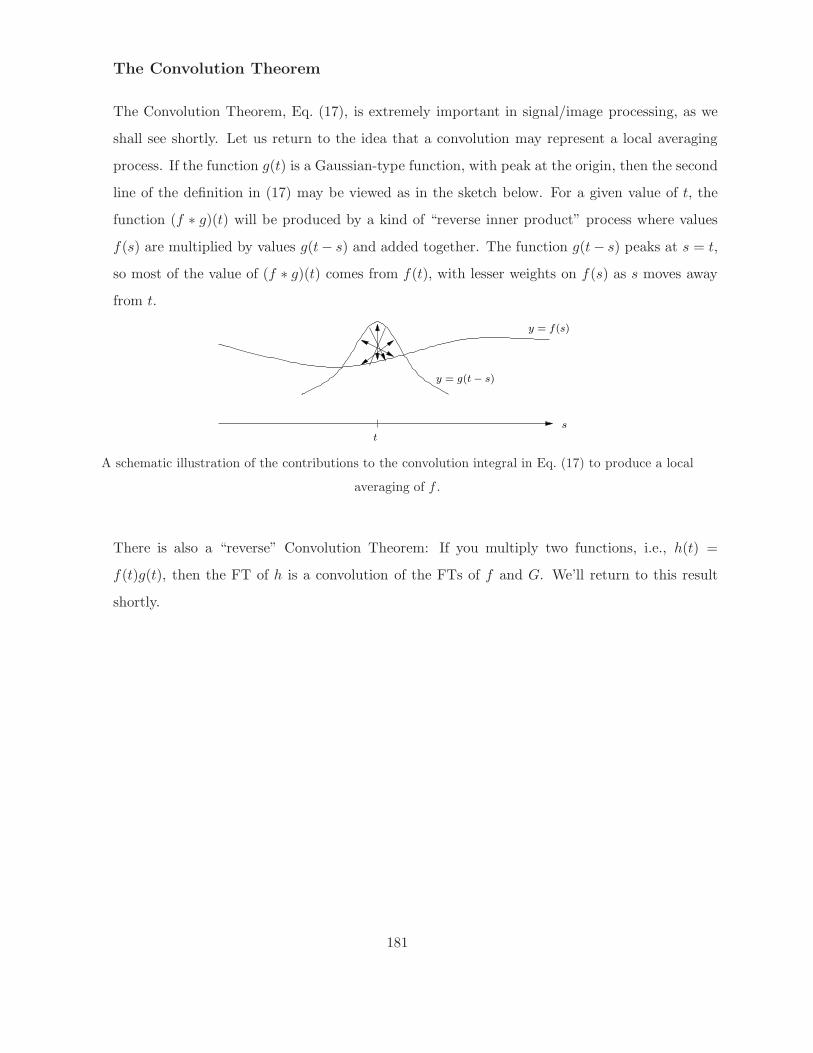
process. If the function g(t) is a Gaussian-type function, with peak at the origin, then the second

line of the definition in (17) may be viewed as in the sketch below. For a given value of t, the

function (f ∗ g)(t) will be produced by a kind of “reverse inner product” process where values

f(s) are multiplied by values g(t− s) and added together. The function g(t − s) peaks at s = t,

so most of the value of (f ∗ g)(t) comes from f(t), with lesser weights on f(s) as s moves away

from t.

y = g(t − s)

y = f(s)

st

A schematic illustration of the contributions to the convolution integral in Eq. (17) to produce a local

averaging of f .

There is also a “reverse” Convolution Theorem: If you multiply two functions, i.e., h(t) =

f(t)g(t), then the FT of h is a convolution of the FTs of f and G. We’ll return to this result

shortly.

181

Lecture 16

Fourier transforms (cont’d)

We continue with a number of important results involving FTs.

Plancherel Formula

Assume that f, g ∈ L2(R). Then

〈f, g〉 = 〈F,G〉, (33)

where 〈·, ·〉 denotes the complex inner product on R, i.e.,

∫

∞

−∞

f(t)g(t) dt =

∫

∞

−∞

F (ω)G(ω) dω. (34)

An important consequence of this result is the following: If f = g, then 〈f, f〉 = 〈F,F 〉, implying that

‖f‖22 = ‖F‖2

2, or ‖f‖2 = ‖F‖2. (35)

This result may also be written as follows,

‖f‖2 = ‖F(f)‖2. (36)

In other words, the symmetric form of the Fourier transform operator is norm-preserving: The L2

norm of f is equal to the norm of F = F(f). (For the unsymmetric forms of the Fourier transform,

we would have to include a multiplicative factor involving 2π or its square root.)

Eq. (35) may be viewed as the continuous version of Parseval’s equation studied earlier in the

context of complete orthonormal bases. Recall the following: Let H be a Hilbert space. If the

orthonormal set {ek}∞0 ⊂ H is complete, then for any f ∈ H,

f =∞∑

k=0

ckek, where ck = 〈f, ek〉, (37)

and

‖f‖L2 = ‖c‖l2 , (38)

i.e.,

‖f‖2 =

∞∑

k=0

|ck|2 (Parseval’s equation). (39)

On the other hand, Parseval’s equation may be viewed as a discrete version of Plancherel’s formula.

182

Proof of Plancherel’s Formula

We first express the function f(t) in terms of the inverse Fourier transform, i.e.,

f(t) =1√2π

∫

∞

−∞

F (ω)eiωtdω. (40)

Now substitute for F (ω) using the definition of the Fourier transform:

f(t) =1

2π

∫

∞

−∞

∫

∞

−∞

f(s)e−iωsds eiωtdω. (41)

Now take the inner product of f(t) with g(t):

〈f, g〉 =

∫

∞

−∞

1

2π

∫

∞

−∞

∫

∞

−∞

f(x)e−iωsds eiωtdω g(t) dt. (42)

We now assume that f and g are sufficiently “nice” so that Fubini’s Theorem will allow us to rearrange

the order of integration. The result is

〈f, g〉 =

∫

∞

−∞

(

1√2π

∫

∞

−∞

f(s)e−iωsds

)(

1√2π

∫

∞

−∞

g(t)eiωtdt

)

dω

=

∫

∞

−∞

F (ω)G(ω) dω,

= 〈F,G〉. (43)

The Fourier transform of a Gaussian (in t-space) is a Gaussian (in ω-space)

This is a fundamental result in Fourier analysis. To show it, consider the following function,

f(t) =1

σ√

2πe−

t2

2σ2 . (44)

You might recognize this function: It is the normalized Gaussian distribution function, or simply the

normal distribution with zero-mean and standard deviation σ or variance σ2. The factor in front of

the integral normalizes it, since

∫

∞

−∞

f(t) dt =1

σ√

2π

∫

∞

−∞

e−t2

2σ2 dt = 1. (45)

(The above result implies that the L1 norm of f is 1, i.e., ‖f‖1 = 1.)

Just in case you are not fully comfortable with this result, we mention that all of these results

come from the following fundamental integral:

∫

∞

−∞

e−x2dx =

√π. (46)

183

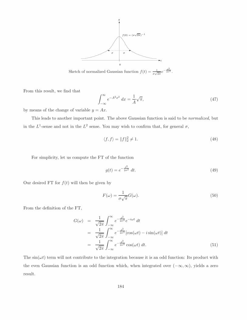
t

f(0) = (σ√

2π)−1

0

y

σ σ

Sketch of normalized Gaussian function f(t) = 1σ√

2πe−

t2

2σ2 .

From this result, we find that∫

∞

−∞

e−A2x2dx =

1

A

√π, (47)

by means of the change of variable y = Ax.

This leads to another important point. The above Gaussian function is said to be normalized, but

in the L1-sense and not in the L2 sense. You may wish to confirm that, for general σ,

〈f, f〉 = ‖f‖22 6= 1. (48)

For simplicity, let us compute the FT of the function

g(t) = e−t2

2σ2 dt. (49)

Our desired FT for f(t) will then be given by

F (ω) =1

σ√

πG(ω). (50)

From the definition of the FT,

G(ω) =1√2π

∫

∞

−∞

e−t2

2σ2 e−iωt dt

=1√2π

∫

∞

−∞

e−t2

2σ2 [cos(ωt) − i sin(ωt)] dt

=1√2π

∫

∞

−∞

e−t2

2σ2 cos(ωt) dt. (51)

The sin(ωt) term will not contribute to the integration because it is an odd function: Its product with

the even Gaussian function is an odd function which, when integrated over (−∞,∞), yields a zero

result.

184

The resulting integral in (51) is not straightforward to evaluate because the antiderivative of the

Gaussian does not exist in closed form. But we may perform a trick here. Let us differentiate both

sides of the equation with respect to the parameter ω. The differentiation of the integrand is permitted

by “Leibniz’ Rule”, so that

G′(ω) = − 1√2π

∫

∞

−∞

te−t2

2σ2 sin(ωt) dt. (52)

The appearance of the “t” in the integrand now permits an antidifferentiation using integration by

parts: Let u = sin(ωt) and dv = −t exp(−t2/(2σ2)), so that v = σ2 exp(−t2/(2σ2)) and du = ω cos(ωt).

Then

G′(ω) =1√2π

[

sin(ωt)e−t2

2σ2

]

∞

−∞

− σ2ω1√2π

∫

∞

−∞

e−t2

2σ2 cos(ωt) dt. (53)

The first term is zero, because the Gaussian function e−t2

2σ2 → 0 as t → ±∞. And the integral on

the right, which once again involves the cos(ωt) function, along with the 1/√

2π factor, is our original

G(ω) function. Therefore, we have derived the result,

G′(ω) = −σ2ωG(ω). (54)

This is a first order DE in the function G(ω). It is also a separable DE and may be easily solved

to yield the general solution (details left for reader):

G(ω) = De−12σ2ω2

, (55)

where D is the arbitrary constant. From the fact that

G(0) =1√2π

∫

∞

−∞

e−t2

2σ2 dt =1√2π

√2πσ = σ, (56)

we have that D = σ, implying that

G(ω) = σe−12σ2ω2

. (57)

From (50), we arrive at our goal, F (ω), the Fourier transform of the Gaussian function

f(t) =1

σ√

2πe−

t2

2σ2 (58)

is

F (ω) =1√2π

e−12σ2ω2

. (59)

As the title of this section indicated, the Fourier transform F (ω) is a Gaussian in the variable ω.

185

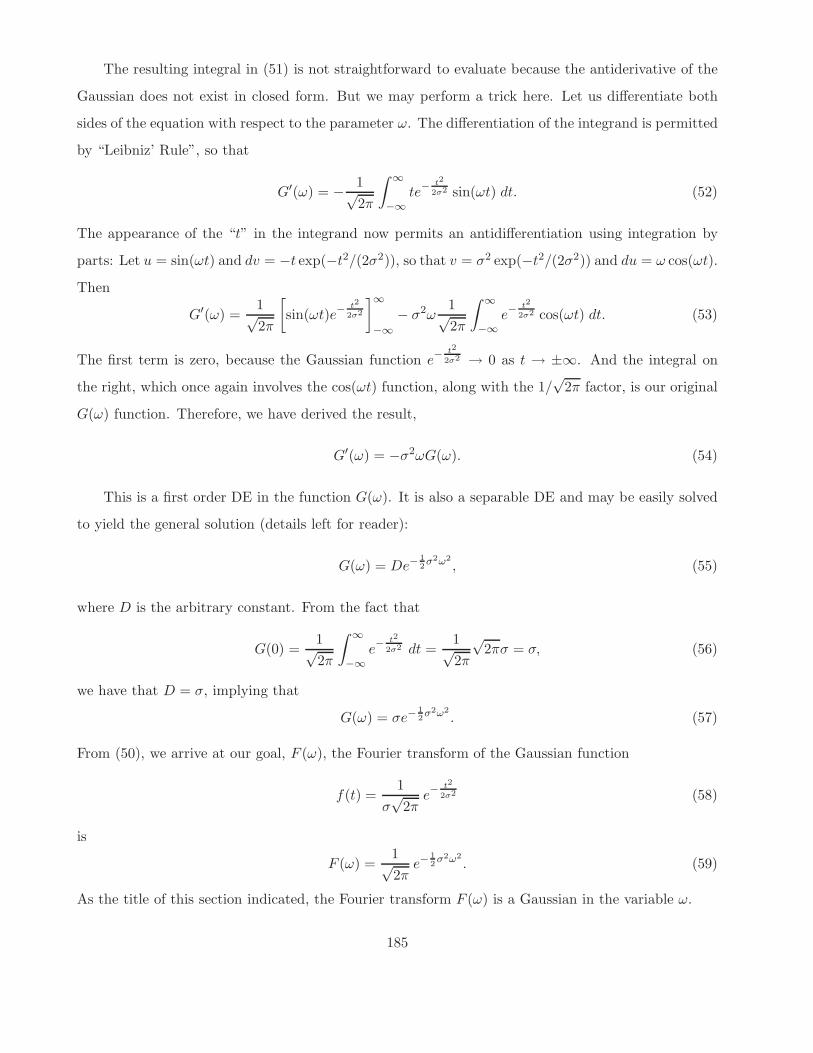
There is one fundamental difference, however, between the two Gaussians, F (ω) and f(t). The

standard deviation of f(t) is σ. But the standard deviation of F (ω), i.e., the value of ω at which F (ω)

assumes the value e−1/2F (0), is σ−1. In other words, if σ is small, so that the Gaussian f(t) is a thin

peak, then F (ω) is broad. This relationship, which is a consequence of the complementarity of the

time (or space) and frequency domains, is sketched below.

t

f(0) = (σ√

2π)−1

0

y

σ σ

0

y

ω1/σ1/σ

Fσ(0) = (√

2π)−1

Generic sketch of normalized Gaussian function fσ(t) = 1σ√

2πe−

t2

2σ2 , with standard deviation σ (left), and its

Fourier transform Fσ(ω) = 1√

2πe−

1

2σ2ω2

with standard deviation 1/σ (right).

Of course, the reverse situation also holds: If σ is large, so that fσ(t) is broad, then 1/σ is small,

so that Fσ(ω) is thin and peaked. These are but special examples of the “Uncertainty Principle” that

we shall examine in more detail a little later.

The limit σ → 0 and the Dirac delta function

Let’s return to the Gaussian function originally defined in Eq. (44),

f(t) =1

σ√

2πe−

t2

2σ2 . (60)

With a little work, it can be shown that in the limit σ → 0,

fσ(t) → 0 t 6= 0, fσ(0) → ∞. (61)

This has the aroma of the “Dirac delta function,” denoted as δ(t). As you may know, the Dirac delta

function is not a function, but rather a generalized function or distribution which must be understood

in the context of integration with respect to an appropriate class of functions. Recall that for any

continuous function g(t) on R, and an a ∈ R

∫

∞

−∞

g(t)δ(t) dt = g(0). (62)

186

It can indeed be shown that

limσ→0

∫

∞

−∞

g(t)fσ(t) dt = g(0) (63)

for any continuous function g(t). As such we may state, rather loosely here, that in the limit σ → 0,

the Gaussian function fσ(t) becomes the Dirac delta function. (There is a more rigorous treatment of

the above equation in terms of “generalized functions” or “distributions”.)

Note also that in the limit σ → 0, the Fourier transform of fσ(t), i.e., the Gaussian function

Gσ(ω), becomes the constant function 1/√

2π. This agrees with the formal calculation of the Fourier

transform of the Dirac delta function δ(t):

F [δ(t)] = ∆(ω) =1√2π

∫

∞

−∞

δ(t)e−iωt dt =1√2π

. (64)

From a signal processing perspective, this is the worst kind of Fourier transform you could have: all

frequencies are present and there is no decay as ω → ±∞. Note that this is not in disagreement with

previous discussions concerning the decay of Fourier transforms since neither the Dirac delta function,

δ(t), nor its Fourier transform, ∆(ω), are L2(R) functions.

Some final notes regarding Dirac delta functions and their occurrence in Fourier

analysis

As mentioned earlier, the “basis” functions eiωt employed in the Fourier transform are not L2(R)

functions. Nevertheless, they may be considered to obey an orthogonality property of the form,

〈eiω1t, eiω2t〉 =

∫

∞

−∞

ei(ω1−ω2)t dt =

0, ω1 6= ω2,

∞, ω1 = ω2,(65)

This has the aroma of a Dirac delta function. But the problem is that the infinity on the RHS is

unchanged if we multiply it by a constant. Is the RHS simply the Dirac delta function δ(ω1 − ω2)?

Or is it a constant times this delta function?

To answer this question, we can go back to the Fourier transform result in Eq. (64). The inverse

Fourier transform associated with this result is

1√2π

∫

∞

−∞

(

1√2π

)

eiωt dω = δ(t), (66)

which implies that1

2π

∫

∞

−∞

eiωt dω = δ(t). (67)

187

Note that there is a symmetry here: We could have integrated eiωt with respect to t to produce a δ(ω)

on the right, i.e.,1

2π

∫

∞

−∞

eiωt dt = δ(ω). (68)

But we can replace ω above by ω1 − ω2, i.e.,

1

2π

∫

∞

−∞

ei(ω1−ω2)t dt = δ(ω1 − ω2). (69)

The left-hand side of the above equation may be viewed as an inner product so that we have the

following orthonormality result,

⟨

1√2π

eiω1t,1√2π

eiω2t

⟩

= δ(ω1 − ω2), ω1, ω2 ∈ R. (70)

In other words, the functions1√2π

eiωt, (71)

with continuous index ω ∈ R, may be viewed as forming an orthonormal set over the real line R

according to the orthonormality relation in Eq. (70).

Note: In Physics, the functions in Eq. (71) are known as plane waves with (angular) frequency ω.

These functions are not square integrable functions on the real line R. In other words, they are not

elements of L2(R).

And just to clean up loose ends, Eq. (70) indicates that the orthogonality relation in Eq. (65)

should be written as

〈eiω1t, eiω2t〉 =

∫

∞

−∞

ei(ω1−ω2)t dt = 2πδ(ω1 − ω2), ω1, ω2 ∈ R, (72)

Finally, it may seem quite strange – and perhaps a violation of Plancherel’s Formula – that in

the limit σ → 0, the area under the curve of the Fourier transform F (ω) becomes infinite, whereas

the area under the curve fσ(t) appears to remain finite. Recall, however, that Plancherel’s Formula

relates the L2 norms of the functions f and g. It is left as an exercise to see what is going on here.

188

The Convolution Theorem revisited – “Convolution Theorem Version 2”

Recall the Convolution Theorem for Fourier transforms: Given two functions f(t) and g(t) with Fourier

transforms F (ω) and G(ω), respectively. Then the Fourier transform of their convolution,

h(t) = (f ∗ g)(t) =

∫

−∞

f(t − s)g(s) ds

=

∫

−∞

f(s)g(t − s) ds, (73)

is given by

H(ω) =√

2πF (ω)G(ω). (74)

Let us now express the above result as follows,

F(f ∗ g) =√

2πFG. (75)

There is a symmetry between the Fourier transform and its inverse that we shall now exploit. With

an eye toward Eqs. (17) and (21), let us now consider a convolution – in frequency space – between

the two Fourier transforms F (ω) G(ω):

(F ∗ G)(ω) =

∫

∞

−∞

F (ω − λ)G(λ) dλ. (76)

We now take the inverse Fourier transform of this convolution, i.e.,

[F−1(F ∗ G)](t) =1√2π

∫

∞

−∞

(F ∗ G)(ω) eiωt dω

=1√2π

∫

∞

−∞

∫

∞

−∞

F (ω − λ)g(λ) dλ eiω dω

=1√2π

∫

∞

−∞

∫

∞

−∞

F (ω − λ)g(λ) dλ ei(ω−λ)eiλ dω

(77)

In the same way as we did before, we consider the change of variable

u(ω, λ) = λ, v(ω, λ) = ω − λ, (78)

with Jacobian J = 1, implying that ω λ = uv. The above integral separates, and the result is, as you

might have guessed,

[F−1(F ∗ G)](t) =√

2πf(t)g(t). (79)

We may also express this result as

F [f(t)g(t)] =1√2π

(F ∗ G)(ω). (80)

189

In other words, the Fourier transform of a product of functions is, up to a constant, the same as

the convolution of their Fourier transforms. We shall refer to this result as Convolution Theorem –

Version 2.

You might well wonder, “When would we be interested in the Fourier transform of a product of

functions?” We’ll return to this question a little later. For the moment, it is interesting to ponder

these two versions of the Convolution Theorem as manifestations of a single theme:

A product of functions in one representation

is equivalent to a convolution in the other.

Using the Convolution Theorem to reduce high-frequency components

As we saw in our discussion of the discrete Fourier transform, many denoising methods work on

the principle of reducing high-frequency components of the noisy signal. Here we examine two sim-

ple methods applied to the Fourier transform which are essentially continuous versions of what was

discussed for DFTs.

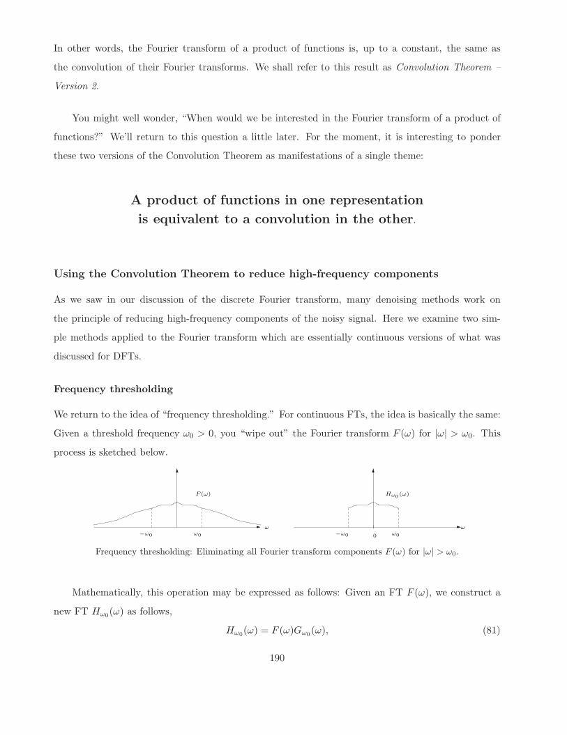
Frequency thresholding

We return to the idea of “frequency thresholding.” For continuous FTs, the idea is basically the same:

Given a threshold frequency ω0 > 0, you “wipe out” the Fourier transform F (ω) for |ω| > ω0. This

process is sketched below.

0

ωω0−ω0

ω−ω0

F (ω) Hω0(ω)

ω0

Frequency thresholding: Eliminating all Fourier transform components F (ω) for |ω| > ω0.

Mathematically, this operation may be expressed as follows: Given an FT F (ω), we construct a

new FT Hω0(ω) as follows,

Hω0(ω) = F (ω)Gω0(ω), (81)

190

where Gω0(ω) is a boxcar-type function,

Gω0(ω) =

1, −ω0 ≤ ω ≤ ω0,

0, otherwise.(82)

From Eq. (81), this has the effect of producing a new signal hω0(t) from f(t) in the following way

hω0(t) =√

2π (f ∗ gω0)(t), (83)

where gω0(t) = F−1[Gω0 ] is a scaled sinc function. (The exact form of Gω0 is left as an exercise.)

Now, if you were faced with the problem of denoising a noisy signal f(t), you have two possibilities

of constructing the denoised signal hω0(t):

1. (i) From f(t), construct its FT F (ω). Then (ii) perform the “chopping operation” of Eq. (81)

to produce Hω0(ω). Finally, (iii) perform an inverse FT on Hω0 to produce hω0(t).

2. For each t, compute the convolution in Eq. (83).

Clearly, the first option represents less computational work. In the second case, you would have to

perform an integration – in practice over N data points – for each value of t. This gives you an

indication of why signal/image processors prefer to work in the frequency domain.

Gaussian weighting

The above method of frequency thresholding, i.e., “chopping the tails of F (ω),” may be viewed as a

rather brutal procedure, especially if many of the coefficients of the tail are not negligible. One may

wish to employ a “smoother” procedure of reducing the contribution of high-frequency components.

One method is to multiply the FT F (ω) with a Gaussian function, which we shall write as follows,

Gκ(ω) = e−ω2

2κ2 . (84)

Note that we have not normalized this Gaussian in order to ensure that that Gκ(0) = 1: For ω near

0, Gκ(ω) ≈ 1, so that low-frequency components of F (ω) are not affected very much. Of course,

by varying the standard deviation κ, we perform different amounts of high-frequency reduction: κ

measures the spread of Gκ(ω) in ω-space.

We denote the Gaussian-weighted FT by

Hκ(ω) = F (ω)Gκ(ω). (85)

191

From the Convolution Theorem, it follows that the resulting signal will be given by

hκ(t) =√

2π (f ∗ gκ0)(t), (86)

where

gκ(t) = F−1[Gκ]. (87)

Note that in this case, the convolution kernel gκ(t) is a Gaussian function. Moreover, the standard

deviation of gκ(t) is 1/κ0. (Remember our derivation that the FT of a Gaussian is a Gaussian, and

vice versa.)

Convolution with a Gaussian is a kind of averaging procedure, where most of the weight is put

at the t-value around which the convolution is being performed. Note that for very large κ, most

of the averaging is performed over a tiny interval centered at each t. Indeed, in the limit κ → ∞,

the averaging will involve only one point, i.e., f(t). This is consistent with the fact that in the limit

κ → ∞, Gκ(ω) = 1, i.e., the Fourier transform F (ω) is left unchanged. As a result, the signal is

unchanged.

On the other hand, for κ very small, i.e., significant damping of higher-frequency components of

F (ω), the averaging of f(t) is performed over a larger domain centered at t.

Once again, it would seem more efficient to perform such a procedure in the frequency domain.

That being said, many image processing packages allow you to perform such Gaussian filtering in

the time or spatial/pixel domain. In the case of images, the result is a blurring, with perhaps some

denoising, of the image.

The Gaussian function Gκ(ω) presented above is but one example of a low-pass filter. (“Low-pass”

means that lower frequencies are allowed to pass through relatively untouched.) Any function G(ω)

that satisfies the following properties,

1. limω→0

G(ω) = 1,

2. G(ω) → 0 as |ω| → ∞,

qualifies as a low-pass filter. (In the next section, the constant 1 will be modified because of the√

2π

factors that occur in the definition of the Fourier transform.)

192

A return to Convolution Theorem - Version 2

We now return to the question, “When would the second version of the Convolution Theorem, i.e.,

F [f(t)g(t)] =1√2π

(F ∗ G)(ω). (88)

which involves the product of two functions f(t) and g(t), be useful/interesting?”

One rather simple situation that may be modelled by the product of two functions is the clipping

of a signal, i.e., taking a signal f(t) defined over R, and setting it to zero outside an interval of interest,

say, [0, T ]. This is quite analogous to the frequency thresholding method discussed earlier.

Setting f(t) to zero outside the interval [0, T ] is equivalent to multiplying f(t) by the boxcar-type

function

g(t) =

1, 0 ≤ t ≤ T,

0, otherwise.(89)

In the frequency domain, the operation h(t) = f(t)g(t) becomes, from the second version of the

Convolution Theorem,

H(ω) =1√2π

(F ∗ G)(ω). (90)

Here G(ω) is a sinc function.

Once again, such a clipping of the signal may be viewed as a rather brutal procedure and the

convolution of its FT, F (ω), with a sinc function attests to this. In fact, an example of this procedure

was already seen in Example No. 2 of Lecture 14, where we “clipped” the function cos 3t and considered

it to be zero outside the interval [−π, π]. The result was a Fourier transform F (ω) - which was explicitly

computed - that was nonzero over the entire real line. The function F (ω) may also be computed by

means of a convolution of a suitable sinc function with the Fourier transform of the function cos 3t.

(The latter is actually a sum of two Dirac delta functions.)

Now that you have produced a function h(t) that is defined on a finite interval [a, b], it is better to

analyze it in terms of Fourier series, i.e., a discrete version of the Fourier transform. This, of course,

will implicitly define a T -periodic extension of h(t). As we have seen earlier in this course, in order

to bypass problems with discontinuities at the endpoints, it is better to consider the even extension

of h(t) to the interval [−T, T ] and then the 2π-periodic extension of this function. This is done by

simply using a Fourier cosine series expansion for h(t), using the data on [0, T ].

The above operation of “clipping” may be considered as a primitive attempt to study the local

properties of f(t) over the interval [0, T ]. From our discussions on frequency damping, one may wish

193

to consider less brutal localizations, for example, the multiplication of f(t) by a Gaussian function

gσ0,t0(t) with variance σ20 and centered at the point t0, i.e.,

h(t) = f(t)gσ0,t0(t). (91)

The Gaussian function g is a kind of “envelope function.” By varying t0, we may examine the properties

of h(t) at various places in the signal. This is the basis of windowed transforms, for example, the so-

called “Gabor transform,” which is essentially a Fourier transform of such a Gaussian modulated

function. We shall examine this method later in the course.

194

Lecture 17

Unfortunately, the Friday, February 15 lecture had to be cancelled. The plan was to present the

following material, which is intended to be supplementary only. You are are not responsible for this

material for the midterm or final examinations. That being said, it is hoped that you will go through

this section because of its relevance to the course. It should give you a bigger picture of the effective-

ness of several areas of mathematics, including Fourier transforms, PDEs and numerical methods in

PDEs, in signal and image processing.

Most of the following material was taken from the instructor’s lecture notes in AMATH 353, Partial

Differential Equations I.

Supplementary reading: The heat equation and the “smoothing” of

signals and images

In AMATH 231, and possibly other courses, you encountered the heat or diffusion equation, a very

important example of a partial differential equation. In the case of a single spatial variable x and

the time variable t, the heat equation for the function u(x, t) has the form

∂u

∂t= k

∂2u

∂x2. (92)

With appropriate boundary conditions and initial conditions, the function u(x, t) could represent the

temperature at a position x of a thin rod at time t.

In the case of three spatial dimensions, the heat equation for the function u(x, t) has the form

∂u

∂t= k∇2u, (93)

where ∇2 denotes the Laplacian operator,

∇2u =∂2u

∂x2+

∂2u

∂y2+

∂2u

∂z2. (94)

Here, the function u(x, t) could represent the temperature at a point x ∈ R3 at time t. Since this

PDE also models diffusion, the function u(x, t) could represent the concentration of a chemical in a

solution.

It is not the purpose here to discuss the heat/diffusion equation in any detail. We simply wish

to show that it is actually relevant to signal and image processing. Historically, it was the Fourier

195

transform solution of the heat equation that inspired a great deal of research into the use of PDEs in

signal and image processing. This research has led to many quite sophisticated mathematical methods

of signal and image processing, including denoising and deblurring.

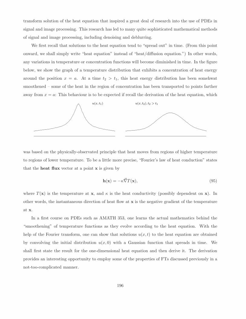
We first recall that solutions to the heat equation tend to “spread out” in time. (From this point

onward, we shall simply write “heat equation” instead of “heat/diffusion equation.”) In other words,

any variations in temperature or concentration functions will become diminished in time. In the figure

below, we show the graph of a temperature distribution that exhibits a concentration of heat energy

around the position x = a. At a time t2 > t1, this heat energy distribution has been somehwat

smoothened – some of the heat in the region of concentration has been transported to points farther

away from x = a: This behaviour is to be expected if recall the derivation of the heat equation, which

u(x, t1) u(x, t2), t2 > t1

was based on the physically-observated principle that heat moves from regions of higher temperature

to regions of lower temperature. To be a little more precise, “Fourier’s law of heat conduction” states

that the heat flux vector at a point x is given by

h(x) = −κ~∇T (x), (95)

where T (x) is the temperature at x, and κ is the heat conductivity (possibly dependent on x). In

other words, the instantaneous direction of heat flow at x is the negative gradient of the temperature

at x.

In a first course on PDEs such as AMATH 353, one learns the actual mathematics behind the

“smoothening” of temperature functions as they evolve according to the heat equation. With the

help of the Fourier transform, one can show that solutions u(x, t) to the heat equation are obtained

by convolving the initial distribution u(x, 0) with a Gaussian function that spreads in time. We

shall first state the result for the one-dimensional heat equation and then derive it. The derivation

provides an interesting opportunity to employ some of the properties of FTs discussed previously in a

not-too-complicated manner.

196

Solution to 1D heat equation by convolution with a Gaussian heat kernel: Given the

heat/diffusion equation on R,

∂u

∂t= k

∂2u

∂x2, −∞ < x < ∞, (96)

with initial condition

u(x, 0) = f(x). (97)

The solution to this initial value problem is

u(x, t) =

∫

∞

−∞

f(s)ht(x − s) ds, t > 0, (98)

where the “heat kernel” function ht(x) is given by

ht(x) =1√

4πkte−x2/4kt, t > 0. (99)

This is a fundamental result – it states that the solution u(x, t) is the spatial convolution of the

functions f(x) and ht(x).

Derivation of the above result: The derivation of Eq. (98) will be accomplished by taking Fourier

transforms of the heat in Eq. 96). But we first have to clearly define what we mean by the Fourier

transform of a solution u(x, t) to the heat equation. At a given time t ≥ 0, the FT of the solution

function u(x, t) is given by

F(u(x, t)) = U(ω, t) =1√2π

∫

∞

−∞

u(x, t)e−iωxdx. (100)

Note that in this case the Fourier transform is given by an integration over the independent

variable “x” and not “t” as was done in previous sections. This means that we may consider the FT

of the solution function u(x, t) as a function of both the frequency variable ω and the time t.

Let us now take Fourier transforms of both sides of the heat equation in (96), i.e.,

F(

∂u

∂t

)

= kF(

∂2u

∂x2

)

, (101)

where we have acknowledged the linearity of the Fourier transform in moving the constant k out of

the transform. It now remains to make sense of these Fourier transforms.

From our definition of the FT in Eq. (100), we now consider∂u

∂tas a function of x and t and

thereby write

F(

∂u

∂t

)

=1√2π

∫

∞

−∞

∂u

∂t(x, t)e−iωxdx. (102)

197

The only t-dependence in the integral on the right is in the integrand u(x, t). As a result, we may

write

F(

∂u

∂t

)

=∂

∂t

[

1√2π

∫

∞

−∞

u(x, t)e−iωxdx

]

=∂

∂tU(ω, t). (103)

In other words, the partial time-derivative of u(ω, t) is simply the partial time-derivative of U(ω, t).

Once again, we can bring the partial derivative operator ∂/∂t outside the integral because it has

nothing to do with the integration over x.

We must now make sense of the right hand side of Eq. (101). Recalling that x is the variable of

integration and time t is simply another variable, we may employ the property for Fourier transforms

of derivatives of functions: Given a function f(x) with Fourier transform F (ω), then

F(f ′(x)) = (−iω)F (ω). (104)

(Note once again that x is our variable of integration now, not t.) Applying this result to our function

u(x, t), we have

F(

∂u

∂x

)

= −iωF(u) = −iωU(ω, t). (105)

We apply this result one more time to obtain the FT of∂2u

∂x2:

F(

∂2u

∂x2

)

= −ω2F(u)

= = ω2U(ω, t). (106)

Now substitute the results of these calculations into Eq. (101) to give

∂U(ω, t)

∂t= −kω2U(ω, t). (107)

Taking Fourier transforms of both sides of the heat equation converts a PDE involving both partial

derivatives in x and t into a PDE that has only partial derivatives in t. This means that we can solve

Eq. (107) as we would an ordinary differential equation in the independent variable t – in essence,

we may ignore any dependence on the ω variable.

The above equation may be solved in the same way as we solve a first-order linear ODE in t.

(Actually it is also separable.) We write it as

∂U(ω, t)

∂t+ kω2U(ω, t) = 0, (108)

198

and note that the integrating factor is I(t) = ekω2t to give

∂

∂t

[

ekω2tU(ω, t)]

= 0. (109)

Integrating (partially) with respect to t yields

ekω2tU(ω, t) = C (110)

which implies that

U(ω, t) = Ce−kω2t. (111)

Here, C is a “constant” with respect to partial differentiation by t. This means that C can be a

function of ω. As such, we’ll write

U(ω, t) = C(ω)e−kω2t. (112)

You can differentiate this expression partially with respect to t to check that it satisfies Eq. (107).

Now notice that at time t = 0,

U(ω, 0) = C(ω). (113)

In other words, C(ω) is the FT of the function u(x, 0). But this is the initial temperature distribution

f(x), i.e.,

C(ω) =1√2π

∫

∞

−∞

f(x)e−iωxdx = F (ω). (114)

Therefore, the solution Eq. (112) may be rewritten as

U(ω, t) = F (ω)e−kω2t. (115)

The solution of the heat equation in (96) may now be obtained by taking inverse Fourier transforms

of the above result, i.e.,

u(x, t) = F−1(U(ω, t)) = F−1(F (ω)e−kω2t). (116)

Note that we must take the inverse FT of a product of FTs. This should invoke the memory of the

Convolution Theorem (Version 1) from Lecture 15:

F(f ∗ g)(x) =√

2π F (ω)G(ω), (117)

which we may rewrite as

F−1(F (ω)G(ω)) =1√2π

(f ∗ g)(x). (118)

199

(Note that we have now used x to denote the independent variable instead of t.) From Eq. (116), the

solution to the heat equation is given by

u(x, t) =1√2π

(f ∗ g)(x) =1√2π

∫

∞

−∞

f(s)g(x − s) ds, (119)

where g(x, t) is the inverse Fourier transform of the function,

G(ω, t) = e−kω2t = e−(kt)ω2. (120)

We have grouped the k and t variables together to form a constant that multiplies the ω2 in the

Gaussian.

The next step is to find g(x, t), the inverse FT of G(ω, t) - recall that t is an auxiliary variable. We

can now invoke another earlier result – that the FT of a Gaussian, this time in x-space, is a Gaussian

in ω-space. In Lecture 16, we showed that the FT of the Gaussian function,

fσ(x) =1

σ√

2πe−

x2

2σ2 , (121)

(note again that we are using x as the independent variable) is

F (ω) =1√2π

e−12σ2ω2

. (122)

We can use this result to find our desired inverse FT of G(ω, t). First note that both fσ(x) and F (ω)

have a common factor 1/√

2π. We now ignore this factor which allows us to write that

F−1(e−12σ2ω2

) =1

σe−

x2

2σ2 . (123)

We now compare Eqs. (122) and (120) and let

1

2σ2 = kt, (124)

which implies that

σ =√

2kt. (125)

We substitute this result into Eq. (123) to arrive at our desired result, namely, that

g(x, t) = F−1(e−ktω2) =

1√2kt

e−x2

4kt . (126)

200

From Eq. (119), and the definition of the convolution, we arrive at our final result for the solution to

the heat equation,

u(x, t) =1√2π

(f ∗ g)(x)

=1√2π

∫

∞

−∞

f(s)g(x − s) ds

=

∫

∞

−∞

f(s)ht(x − s) ds, (127)

where

ht(x) =1√2π

g(x, t) =1√

4πkte−x2/4kt (128)

denotes the so-called heat kernel. This concludes the derivation.

The heat kernel ht(x) is a Gaussian function that “spreads out” in time: its standard deviation is

given by σ(t) =√

2kt. The convolution in Eq. (127) represents a weighted averaging of the function

f(s) about the point x – as time increases, this weighted averaging includes more points away from

x, which accounts for the increased smoothing of the temperature distribution u(x, t).

In the figure below, we illustrate how a discontinuity in the temperature function gets smoothened

into a continuous distribution. At time t = 0, there is a discontinuity in the temperature function

u(x, 0) = f(x) at x = a. Recall that we can obtain all future distributions u(x, t) by convolving f(x)

with the Gaussian heat kernel. For some representative time t > 0, but not too large, three such

Gaussian kernels are shown at points x1 < a, x2 = a and x3 > a. Since t is not too large, the Gaussian

kernels are not too wide. A convolution of u(x, 0) with these kernels at x1 and x3 will not change the

distribution too significantly, since u(x, 0) is constant over most of the region where these kernels have

significant values. However, the convolution of u(x, 0) with the Gaussian kernel centered at the point

of discontinuity x = x2 will involve values of u(x, 0) to the left of the discontinuity as well as values of

u(x, 0) to the right. This will lead to a significant averaging of the temperature values, as shown in

the figure. At a time t2 > t1, the averaging of u(x, 0) with even wider Gaussian kernels will produce

even greater smoothing.

The smoothing of temperature functions (and image functions below) can also be seen by looking

at what happens in “frequency space,” i.e., the evolution of the Fourier transform U(ω, t) of the

solution u(x, t), as given in Eq. (115), which we repeat below:

U(ω, t) = F (ω)e−kω2t, t ≥ 0. (129)

201

x3a a

t1 > 0

u(x, t), t > 0u(x, 0)

t2 > t1

x1

At any fixed frequency ω > 0, as t increases, the multiplicative Gaussian term e−kω2t decreases, im-

plying that the frequency component, U(ω, t), decreases. For higher ω values, this decrease is faster.

Therefore, higher frequencies are dampened more quickly than lower frequencies. We saw this phe-

nomenon at the end of the the previous lecture.

We now move away from the idea of the heat or diffusion equation modelling the behaviour of

temperatures or concentrations. Instead, we consider the function u(x, t), x ∈ R, as representing a

time-varying signal. And in the case of two spatial dimensions, we may consider the function u(x, y, t)

as representing the time evolution of an image. Researchers in the signal and image processing noted

the smoothing behaviour of the heat/diffusion equation quite some time ago and asked whether it

could be exploited to accomplish desired tasks with signals and images. We outline some of these

ideas very briefly below for the case of images, since the results are quite dramatic visually.

First of all, images generally contain many points of discontinuity – these are the edges of the

image. In fact, edges are considered to define an image to a very large degree, since the boundaries

of any objects in the image produce edges. In what follows, we shall let the function u(x, y, t) denote

the evolution of a (non-negative) image function under the heat/diffusion equation,

∂u

∂t= k∇2u = k

[

∂2u

∂x2+

∂2u

∂y2

]

, u(x, y, 0) = f(x, y). (130)

Here we shall not worry about the domain of definition of the image. In practice, of course, image

functions are defined on a finite set, e.g., the rectangular region [a, b] × [c, d] ⊂ R2.

Some additional notes on the representation of images

Digitized images are defined over a finite set of points in a rectangular domain. Therefore,

they are essentially m × n arrays of greyscale or colour values – the values that are used

202

to assign brightness values to pixels on a computer screen. In what follows, we may

consider such matrices to define images that are piecewise constant over a region of R2.

We shall also be looking only at black-and-white (BW) images. Mathematically, we may

consider the range of greyscale values of a BW image function to be an interval [A,B], with

A representing black and B representing white. In mathematical analysis, one usually

assumes that [A,B] = [0, 1]. As you probably know, the practical storage of digitized

images also involves a quantization of the greyscale values into discrete values. For so-

called “8 bit-per-pixel” BW images, where each pixel may assume one of 28 = 256 discrete

values (8 bits of computer memory are used to the greyscale value at each pixel), the

greyscale values assume the values (black) 0, 1, 2, · · · , 255 (white). This greyscale range,

[A,B] = [0, 255] is used for the analysis and display of the images below.

From our earlier discussions, we expect that edges of the input image f(x, y) will become more

and more smoothened as time increases. The result will be an increasingly blurred image, as we show

in Figure 1 below. The top image in the figure is the input image f(x, y). The bottom row shows

the image u(x, y, t) for two future times. The solutions u(x, y, t) we computed by means of a 2D

finite-difference scheme using forward time difference and centered difference for the Laplacian. It

assumes the following form,

u(n+1)ij = u

(n)ij + s[u

(n)i−1,j + u

(n)i+1,j + u

(n)i,j−1 + u

(n)i,j+1 − 4u

(n)ij ], s =

k∆t

(∆x)2. (131)

(For details, you may consult the text by Haberman, Chapter 6, p. 253.) This scheme is numerically

stable for s < 0.25: The value s = 0.1 was used to compute the images in the figure.

Heat/diffusion equation and “deblurring”

You may well question the utility of blurring an image: Why would one wish to degrade an image in

this way? We’ll actually provide an answer very shortly but, for the moment, let’s make use of the

blurring result in the following way: If we know that an image is blurred by the heat/diffusion equation

as time increases, i.e., as time proceeds forward, then perhaps a blurry image can be deblurred by

letting it evolve as time proceeds backward. The problem of “image deblurring” is an important one,

e.g., acquiring the license plate numbers of cars that are travelling at a very high speed.

If everything proceeded properly, could a blurred edge could possibly be restored by such a pro-

cedure? In theory, the answer is “yes”, provided that the blurred image is known for all (continuous)

203

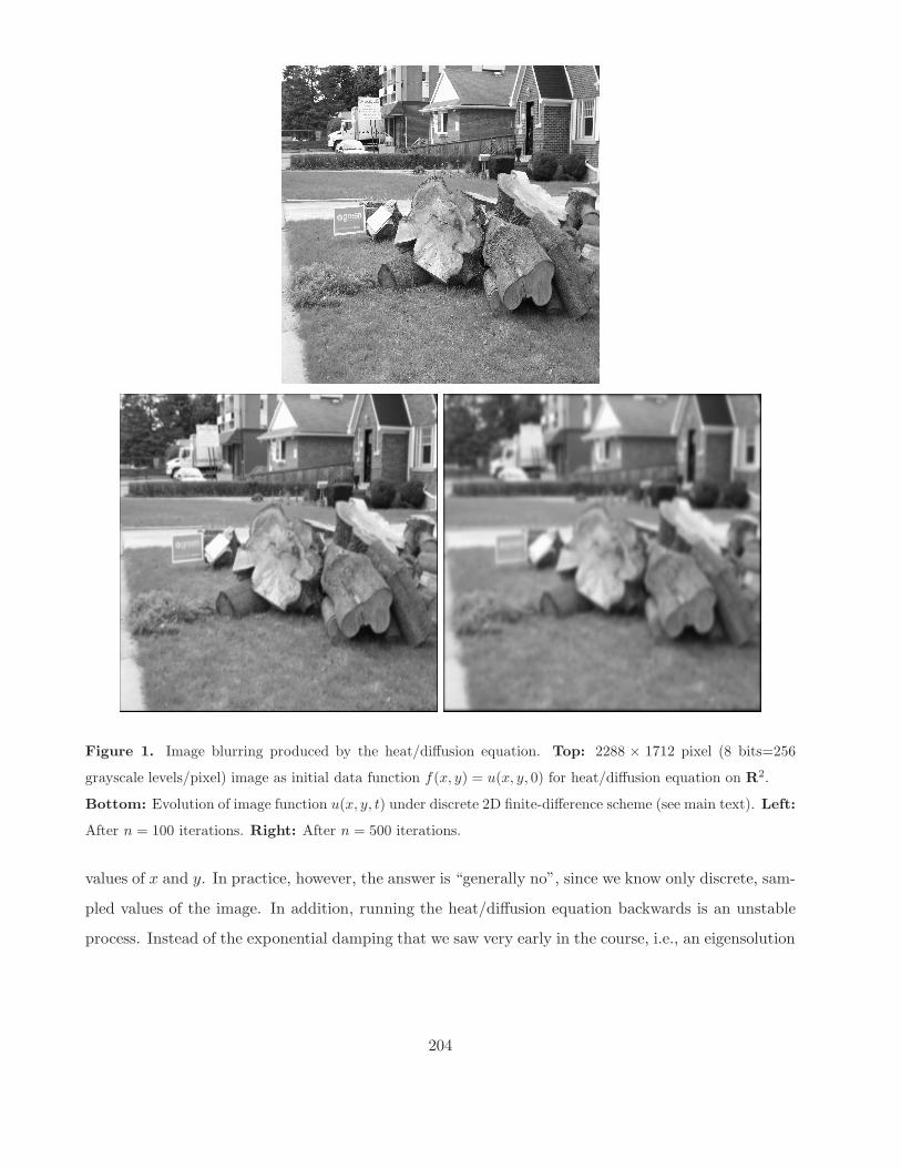
Figure 1. Image blurring produced by the heat/diffusion equation. Top: 2288 × 1712 pixel (8 bits=256

grayscale levels/pixel) image as initial data function f(x, y) = u(x, y, 0) for heat/diffusion equation on R2.

Bottom: Evolution of image function u(x, y, t) under discrete 2D finite-difference scheme (see main text). Left:

After n = 100 iterations. Right: After n = 500 iterations.

values of x and y. In practice, however, the answer is “generally no”, since we know only discrete, sam-

pled values of the image. In addition, running the heat/diffusion equation backwards is an unstable

process. Instead of the exponential damping that we saw very early in the course, i.e., an eigensolution

204

in one dimension, un(x, t) = φnhn(t) evolving as follows,

un(x, t) = φn(x)e−k(nπ/L)2t, (132)

we encounter exponential increase: replacing t with −t yields,

un(x, t) = φn(x)ek(nπ/L)2t. (133)

As such, any inaccuracies in the function will be amplified. As a result, numerical procedures associated

with running the heat/diffusion equation backwards are generally unstable.

To investigate this effect, the blurred image obtained after 100 iterations of the first experiment

was used as the initial data for a heat/diffusion equation that was run backwards in time. This may

be done by changing ∆t to −∆t in the finite difference scheme, implying that s is replaced by −s.

The result is the following “backward scheme,”

u(n−1)ij = u

(n)ij − s[u

(n)i−1,j + u

(n)i+1,j + u

(n)i,j−1 + u

(n)i,j+1 − 4u

(n)ij ]. (134)

The first blurred image of the previous experiment (lower left image of Figure 1) was used as input

into the above backward-time scheme. It is shown at the top of Figure 2. After five iterations, the

image at the lower left of Figure 2 is produced. Some deblurring of the edges has been accomplished.

(This may not be visible if the image is printed on paper, since the printing process itself introduces

a degree of blurring.) After another five iterations, additional deblurring is achieved at some edges

but at the expense of some severe degradation at other regions of the image. Note that much of the

degradation occurs at smoother regions of the image, i.e., where spatially neighbouring values of the

image function are closer to each other. This degradation is an illustration of the numerical instability

of the backward-time procedure.

Image denoising under the heat/diffusion equation

We now return to the smoothing effect of the heat/diffusion equation and ask whether or not it could

be useful. The answer is “yes” – it may be useful in the denoising of signals and/or images. In many

applications, signals and images are degraded by noise in a variety of possible situations, e.g., (i)

atmospheric disturbances, particularly in the case of images of the earth obtained from satellites or

astronomical images obtained from telescopes, (ii) the channel over which such signals are transmitted

are noisy, These are part of the overall problem of signal/image degradation which may include both

205

Figure 2. Attempts to deblur images by running the heat/diffusion equation backwards. Top: Blurred image

u(100)ij from previous experiment, as input into “backward” heat/diffusion equation scheme, with s = 0.1.

Bottom left: Result after n = 5 iterations. Some deblurring has been achieved. Bottom right: Result

after n = 10 iterations. Some additional deblurring but at the expense of degradation in some regions due to

numerical instabilities.

blurring as well as noise. The removal of such degradations, which is almost always only partial, is

known as signal/image enhancement.

A noisy signal may look something like the sketch at the left of Figure 3 below. Recalling that

the heat/diffusion equation causes blurring, one might imagine that the blurring of a noisy signal may

206

produce some deblurring, as sketched at the right of Figure 3. This is, of course, a very simplistic

idea, but it does provide the starting point for a number of signal/image denoising methods.

Denoised image u(x, t)Noisy image f(x) = u(x, 0)

A noisy signal (left) and its denoised counterpart (right).

In Figure 4 below, we illustrate this idea as applied to image denoising. The top left image is our

original, “noiseless” image u. Some noise was added to this image to produce the noisy image u at

the top right. Very simply,

u(i, j) = u(i, j) + n(i, j), (135)

where n(i, j) ∈ R was chosen randomly from the real line according to the normal Gaussian distribution

N (0, σ), i.e., zero-mean and standard deviation σ. In this case, σ = 20 was used. The above equation

is usually written more generally as follows,

u = u + N (0, σ). (136)

For reference purposes, the (discrete) L2 error between u and u was computed as follows,

‖u − u‖2 =

√

√

√

√

1

5122

512∑

i,j=1

[u(i, j) − u(i, j)]2 = 20.03. (137)

This is the “root mean squared error” (RMSE) between the discrete functions u and u. (You first

compute the average value of the squares of the differences of the greyscale values at all pixels. Then

take the square root of this average value.) In retrospect, it should be close to the standard deviation

σ of the added noise. In other words, the average magnitude of the error between u(i, j) and u(i, j)

should be the σ-value of the noise added.

The noisy image u was then used as the input image for the diffusion equation, more specifically,

the 2D finite difference scheme used earlier, i.e.,

u(n+1)ij = u

(n)ij + s[u

(n)i−1,j + u

(n)i+1,j + u

(n)i,j−1 + u

(n)i,j+1 − 4u

(n)ij ], (138)

with s = 0.1.

207

After five iterations (lower left), we see that some denoising has been produced, but at the expense

of blurring, particularly at the edges. The L2 distance between this denoised/blurred image and the

original noiseless image u is computed to be

‖u5 − u‖2 = 16.30. (139)

We see that from the viewpoint of L2 distance, i.e., the denoised image u5 is “closer” to the noiseless

image u than the noisy image u. This is a good sign – we would hope that the denoising procedure

would produce an image that is closer to u. But more on this later.

After another five iterations, as expected, there is further denoising but accompanied by additional

blurring. The L2 distance between this image and u is computed to be

‖u10 − u‖2 = 18.23. (140)

Note that the L2 distance of this image is larger than that of u5 – in other words, we have done worse.

One explanation is that the increased blurring of the diffusion equation has degraded the image farther

away from u than the denoising has improved it.

We now step back and ask: Which of the above results is “better” or “best”? In the L2 sense, the

lower left result is better since its L2 error (i.e., distance to u) is smaller. But is it “better” visually?

Quite often, a result that is better in terms of L2 error is is poorer visually. And are the denoised

images visually “better” than the noisy image itself. You will recall that some people in class had the

opinion that the noisy image u actually looked better than any of the denoised/blurred results. This

illustrates an important point about image processing – the L2 distance, although easy to work with,

is not necessarily the best indicator of visual quality. Psychologically, our minds are sometimes more

tolerant of noise than degradation in the edges – particularly in the form of blurring – that define an

image.

Image denoising using “anisotropic diffusion”

We’re not totally done with the idea of using the heat/diffusion equation to remove noise by means

of blurring. Once upon a time, someone got the idea of employing a “smarter” form of diffusion –

one which would perform blurring of images but which would leave their edges relatively intact. We

could do this by making the diffusion parameter k to be sensitive to edges – when working in the

vicinity of an edge, we restrict the diffusion so that the edges are not degraded. As we mentioned

earlier, edges represent discontinuities – places where the magnitudes of the gradients become quite

208

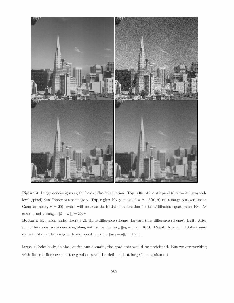
Figure 4. Image denoising using the heat/diffusion equation. Top left: 512× 512 pixel (8 bits=256 grayscale

levels/pixel) San Francisco test image u. Top right: Noisy image, u = u+N (0, σ) (test image plus zero-mean

Gaussian noise, σ = 20), which will serve as the initial data function for heat/diffusion equation on R2. L2

error of noisy image: ‖u − u‖2 = 20.03.

Bottom: Evolution under discrete 2D finite-difference scheme (forward time difference scheme), Left: After

n = 5 iterations, some denoising along with some blurring, ‖u5 − u‖2 = 16.30. Right: After n = 10 iterations,

some additional denoising with additional blurring, ‖u10 − u‖2 = 18.23.

large. (Technically, in the continuous domain, the gradients would be undefined. But we are working

with finite differences, so the gradients will be defined, but large in magnitude.)

209

This implies that the diffusion parameter k would depend upon the position (x, y). But this is

only part of the process – since k would be sensitive to the gradient ~∇u(x, y) of the image, it would,

in fact, be dependent upon the image function u(x, y) itself!

One way of accomplishing this selective diffusion, i.e., slower at edges, is to let k(x, y) be inversely

proportional to some power of the gradient, e.g.,

k = k(‖~∇u‖) = C‖~∇u‖−α, α > 0. (141)

The resulting diffusion equation,∂u

∂t= k(‖~∇u‖)∇2u, (142)

would be a nonlinear diffusion equation, since k is now dependent upon u, and it multiplies the

Laplacian of u. And since the diffusion process is no longer constant throughout the region, it is

no longer homogeneous but nonhomogeneous or anisotropic. As such, Eq. (142) is often called the

anisotropic diffusion equation.

To illustrate this process, we have considered a very simple example, where

k(‖~∇u‖) = ‖~∇u‖−1/2. (143)

Some results are presented in Figure 5. This simply anisotropic scheme works well to preserve edges,

therefore producing better denoising of the noisy image used in the previous experiment. The denoised

image u20 is better not only in terms of L2 distance but also from the perspective of visual quality

since its edges are better preserved.

Needless to say, a great deal of research has been done on nonlinear, anisotropic diffusion and its

applications to signal and image processing.

210

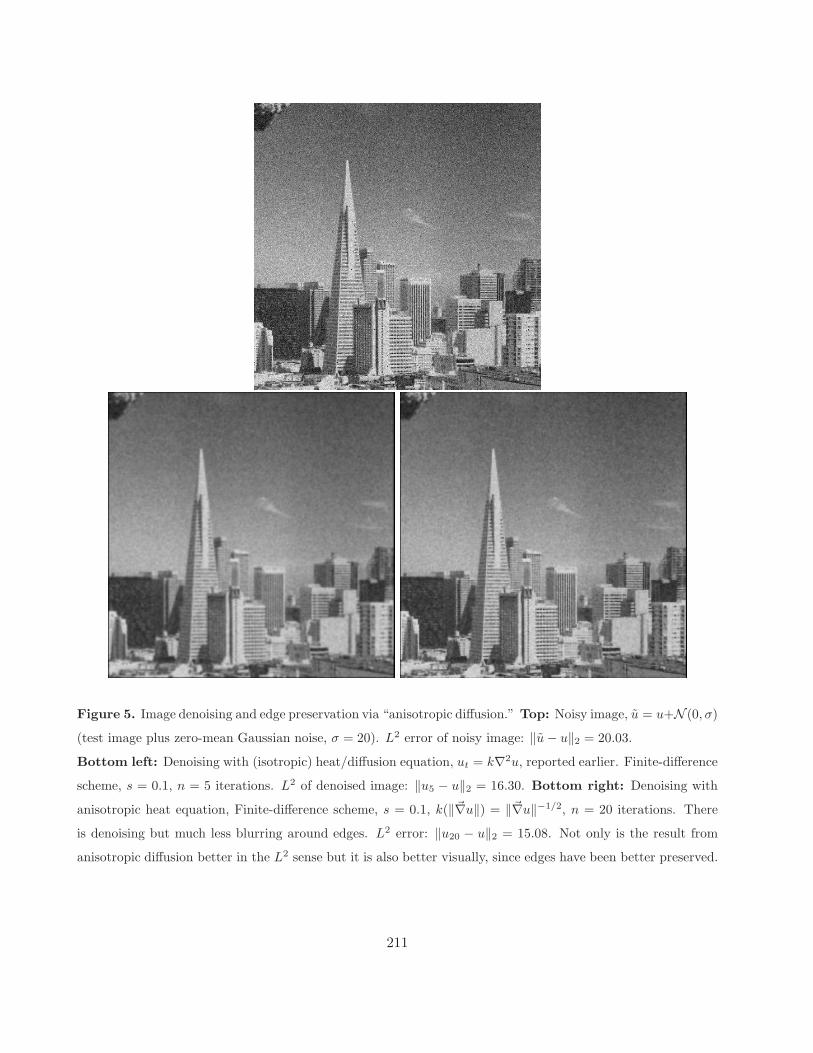
Figure 5. Image denoising and edge preservation via “anisotropic diffusion.” Top: Noisy image, u = u+N (0, σ)

(test image plus zero-mean Gaussian noise, σ = 20). L2 error of noisy image: ‖u − u‖2 = 20.03.

Bottom left: Denoising with (isotropic) heat/diffusion equation, ut = k∇2u, reported earlier. Finite-difference

scheme, s = 0.1, n = 5 iterations. L2 of denoised image: ‖u5 − u‖2 = 16.30. Bottom right: Denoising with

anisotropic heat equation, Finite-difference scheme, s = 0.1, k(‖~∇u‖) = ‖~∇u‖−1/2, n = 20 iterations. There

is denoising but much less blurring around edges. L2 error: ‖u20 − u‖2 = 15.08. Not only is the result from

anisotropic diffusion better in the L2 sense but it is also better visually, since edges have been better preserved.

211