Lecture 13 dr. P. Nazarov -...

edu.sablab.net/transcriptData analysis in trascriptomics 1

dr. P. Nazarov

[email protected]

Lecture 13


Outline

Public data repositories

GEO, ArrayExpress

TCGA

Microarray data

2-,1-color arrays

normalization

RNA-Seq

Exploratory data analysis

PCA

clustering

Differential expression analysis

multiple hypotheses

linear models

Classification and marker genes

Enrichment analysis


Basic Expression Scheme

MICROARRAY DATA ANALYSIS


Basic Expression Scheme

transcription

pre-mRNAintron

DNA G E N E

intronexon 1 exon 2

mRNA

RNA splicing

protein

translation



Alternative Splicing

3 541 2

Heart muscle

1 543Uterine muscle

1 532

Multiple introns may be spliced differently in different circumstances, for

example in different tissues.

Thus one gene can encode more than one protein. The proteins are similar but not

identical and may have distinct properties – an important feature for complex

organisms



Probes

3 541 2

ATTCGACGGCATAAACGGCATAA

CTATTCG

CTATTCGACGGCATAACCTAATG



Data Overview


Public Repositories

GEO: http://www.ncbi.nlm.nih.gov/gds

ArrayExpress: http://www.ebi.ac.uk/arrayexpress/

TCGA: https://tcga-data.nci.nih.gov/tcga/

Sep 2014 – more then 10k patients

Analysis via:http://www.cbioportal.org/public-portal/

Data for our course: http://edu.sablab.net/transcript

http://edu.sablab.net/transcript


Microarray Data

Types of Microarrays

Two-color Arrays (2C)Agilent full genomeThematic arrays

ProDirect comparisonLess sensitive to inaccuracies of

spotting

ConDye effects: need for “dye-swaps”Non-flexibility in analysis

One-color Arrays (1C)Affymetrix GeneChipAffymetrix ExonAffymetrix mRNA

ProFlexible analysisHigh level of standardization

ConPrice


Microarray Data

Two-color Arrays

MAIA

Several spots with the same probe sequence Quantify each spot by a set of parametersFind an optimal rule to accept the spotsRemove bad spots from further analysis

Solutions

LogFC 2

http://bioinfo-out.curie.fr/projects/maia/index.php

𝐿𝑜𝑔 𝑅𝑎𝑡𝑖𝑜 = 𝑙𝑜𝑔𝐹𝐶 = 𝑀 = 𝑙𝑜𝑔2𝑅−𝑅𝑏𝑔

𝐺−𝐺𝑏𝑔=

= 𝑙𝑜𝑔2 𝑅 − 𝑅𝑏𝑔 − 𝑙𝑜𝑔2 𝐺 − 𝐺𝑏𝑔

Measure: red (R) and green (G) fluorescence

Estimate: background fluorescence Rbg , Gbg

𝐿𝑜𝑔 𝐼𝑛𝑡𝑒𝑛𝑐𝑖𝑡𝑦 = 𝐴 =1

2𝑙𝑜𝑔2 𝑅 − 𝑅𝑏𝑔 + 𝐺 − 𝐺𝑏𝑔

Advanced image analysis and corrections are needed


Microarray Data

Normalization of Two-color Arrays

Non-linear dye-effect photodegradation, radiationless energy transfer, quenching

Solution. Lowess (loess) correction

Linear effects b/w samplesdifference in concentration or hybridization efficiency

Solution. Linear centring/scaling


Microarray Data

Normalization of Two-color Arrays

Spatial effectsdue to technological problems

Solution. Spatial normalizationUsing spikes (Agilent)Using numerical methods to estimate 2D profile


Microarray Data

Two-color Array Data Overview

Original LogRatio (logFC)

Original Log Intensity

Normalized Log Ratio (logFC)


Microarray Data

One-color Arrays

High reproducibility and quality of spotting is required.Affymetrix – “photolithography”-like technique

𝐿𝑜𝑔𝐼𝑛𝑡𝑒𝑛𝑠𝑖𝑡𝑦 = 𝑙𝑜𝑔2 𝐼

Background is “removed” during normalization step

Filtering may help removing uninformative features

Raw Normalized


Microarray Data

Affymetrix: Probes, Probesets and Transcript clusters

In old versions of Affy arrays (hgu95, hgu133, etc), there were: PM – perfect match probesMM – mismatch probes (having replacement in th 13th character)This was done for background estimation. But this approach is not used now!!

Probes25-mer sequences

targeted on a single region of transcriptome

(hopefully)

Probesetsgroups of closely located or overlapped probes (on

average 4 probes)

Transcript clustersFor majority of features -synonymous to “genes”. However, some distinct transcripts of genes are considered as different

transcript clusters.

ExonsHuExon and HTA

arrays allow measuring exon

expression

Okoniewski M, Comprehensive Analysis of AffymetrixExon Arrays Using BioConductor, PLoS CompBiol, 2008


Microarray Data

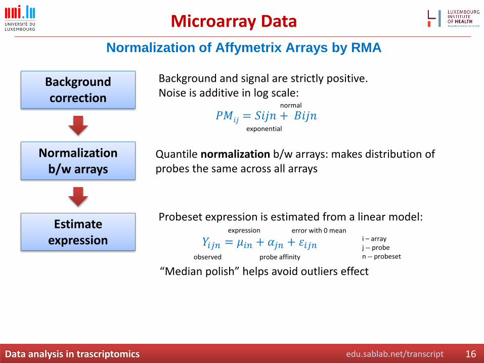
Normalization of Affymetrix Arrays by RMA

Background correction

Background and signal are strictly positive. Noise is additive in log scale:

Normalization b/w arrays

Estimate expression

Quantile normalization b/w arrays: makes distribution of probes the same across all arrays

𝑌𝑖𝑗𝑛 = 𝜇𝑖𝑛 + 𝛼𝑗𝑛 + 𝜀𝑖𝑗𝑛observed probe affinity

expression error with 0 meani – arrayj -- proben -- probeset

Probeset expression is estimated from a linear model:

𝑃𝑀𝑖𝑗 = 𝑆𝑖𝑗𝑛 + 𝐵𝑖𝑗𝑛exponential

normal

“Median polish” helps avoid outliers effect


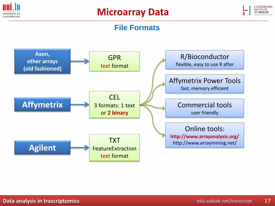
Microarray Data

File Formats

Axon, other arrays

(old fashioned)

Affymetrix

Agilent

GPRtext format

CEL3 formats: 1 text

or 2 binary

TXTFeatureExtraction

text format

R/Bioconductorflexible, easy to use R after

Affymetrix Power Toolsfast, memory efficient

Commercial toolsuser friendly

Online tools:http://www.arrayanalysis.org/http://www.arraymining.net/


Microarray Data

Analysis Pipeline

Image Analysis

Pre-processing

Raw CEL files

Quality control

Statistical Analysis

Text files with log2

gene (or probeset) expression

Lists of differentially

expressed gene

Affymetrix©

software Background

correction Normalization Summarization

Remove low quality arrays,

if necessary

Significance analysis fordifferentially expressed genes (DEG)

Prediction analysis Co-regulation analysis Etc.

Bioinformatics


Microarray Data

Example: Affymetrix Power Tools

apt-probeset-summarize is a program for doing background subtraction, normalization and summarizing probe sets from Affymetrix expression microarrays. It implements analysis algorithms such as RMA, Plier, and DABG (detected above background).The main features of apt-probeset-summarize not common in other implementations are:Quantile normalization using a subset (sketch) of the data which results in much smaller memory usage.

http://www.affymetrix.com/support/developer/powertools/changelog/apt-probeset-summarize.html

apt-probeset-summarize

-a rma-sketch -d chip.cdf -o output-dir --cel-files files.txt

CEL

CDF

CELCEL

files.txt

CEL

apt-probeset-

summarize

TXT table

CSV annotation


http://www.ncbi.nlm.nih.gov/entrez/query.fcgi?db=pubmed&cmd=Retrieve&dopt=AbstractPlus&list_uids=12582260&query_hl=2&itool=pubmed_docsum

http://www.affymetrix.com/support/technical/technotes/plier_technote.pdf



RNA-Seq Data

Next Generation Sequencing: RNA-Seq

Wang Z et al. RNA-Seq: a revolutionary tool for transcriptomics. Nat Rev Genet. 2009

raw counts

coverage

normalized counts: CPM, fpkm, rpkm


RNA-Seq Data

File Types

Raw image files

FASTQ files

SAM/BAM files

Mapping

@HWI-ST508:152:D06G9ACXX:2:1101:1160:2042 1:Y:0:ATCACG

NAAGACCGAATTCTCCAAGCTATGGTAAACATTGCACTGGCCTTTCATCTG

+

#11??+2<<<CCB4AC?32@+1@AB1**1?AB<4=4>=BB<9=>?######

@HD VN:1.0 SO:coordinate

@SQ SN:seq1 LN:5000

@SQ SN:seq2 LN:5000

@CO Example of SAM/BAM file format.

B7_591:4:96:693:509 73 seq1 1 99 36M *

0 0 CACTAGTGGCTCATTGTAAATGTGTGGTTTAACTCG

<<<<<<<<<<<<<<<;<<<<<<<<<5<<<<<;:<;7

MF:i:18 Aq:i:73 NM:i:0 UQ:i:0 H0:i:1

H1:i:0EAS54_65:7:152:368:113 73 seq1 3 99

35M * 0 0

CTAGTGGCTCATTGTAAATGTGTGGTTTAACTCGT

<<<<<<<<<<0<<<<655<<7<<<:9<<3/:<6): MF:i:18 Aq:i:66

NM:i:0 UQ:i:0 H0:i:1 H1:i:0

Counting

Raw counts

Normalized countscpm, fpkm, rpkm For the list of tools see:

http://en.wikipedia.org/wiki/List_of_RNA-Seq_bioinformatics_tools

Read – a short sequence identified in RNA-Seq experimentLibrary – set (105 – 108) of reads from a single sample


RNA-Seq

Normalization

Problems:

Libraries has different size (different number of reads from samples)

Long transcripts produce more reads

Solutions (?) :

Accounting for library size during analysis (standard) or direct correction for it

Correction for transcript size (but which transcript is expressed?)

Corrected?..


Exploratory Analysis


Exploratory Data Analysis

Principal Component Analysis (PCA)

Principal component analysis (PCA)is a vector space transform used to reduce multidimensional data sets to lower dimensions for analysis. It selects the coordinates along which the variation of the data is bigger.

Variable 1

Var

iab

le 2

Scatter plot in “natural” coordinates

Scatter plot in PC

First component

Seco

nd

co

mp

on

ent

Instead of using 2 “natural” parameters for the classification, we can use the first component!

20000 genes 2 dimensions

For the simplicity let us consider 2 parametric situation both in terms of data and resulting PCA.



PCA



PCA in TCGA (LUSC data)

Healthy

Cancer



k-Means Clustering

k-Means Clusteringk-means clustering is a method of cluster analysis which aims to partition n observations into k clusters in which each observation belongs to the cluster with the nearest mean.

1) k initial "means" (in this case k=3) are randomly selected from the data set (shown in color).

2) k clusters are created by associating every observation with the nearest mean.

3) The centroid of each of the k clusters becomes the new means.

4) Steps 2 and 3 are repeated until convergence has been reached.

http://wikipedia.org



k-Means Clustering: Iris Dataset (Fisher)

clusters = kmeans(x=Data,centers=3,nstart=10)$cluster

plot(PC$x[,1],PC$x[,2],col = classes,pch=clusters)

legend(2,1.4,levels(iris$Species),col=c(1,2,3),pch=19)

legend(-2.5,1.4,c("c1","c2","c3"),col=4,pch=c(1,2,3))

-3 -2 -1 0 1 2 3 4

-1.0

-0.5

0.0

0.5

1.0

PC$x[, 1]

PC

$x[, 2

]

setosa

versicolor

virginica

c1

c2

c3



Hierarchical Clustering

Hierarchical ClusteringHierarchical clustering creates a hierarchy of clusters which may be represented in a tree structure called a dendrogram. The root of the tree consists of a single cluster containing all observations, and the leaves correspond to individual observations.Algorithms for hierarchical clustering are generally either agglomerative, in which one starts at the leaves and successively merges clusters together; or divisive, in which one starts at the root and recursively splits the clusters.

http://wikipedia.orgDistance: Euclidean

Elements

Agg

lom

erat

ive D

ivisive

Dendrogram



Heatmaps



Fuzzy Clustering: Mfuzz


Differential Expression

Analysis


Differential Expression Analysis

Basics

Questions

Which genes have changes in mean expression level between conditions?

How reliable are this observations

DEA

Single factor, two conditions

Similar to t-test with Student’s statistics: compare means

Multifactor or multicondition

Similar to ANOVA with Fisher’s statistics: compare variances

Post-hoc analysis

Example: 2 cell lines in time:

And do not forget about multiple hypotheses testing



34

Example

http://www.xkcd.com/882/



Multiple Hypotheses

False Positive,

error

False Negative,

error

Probability of an error in a multiple test:

1–(0.95)number of comparisons



Multiple Hypotheses: False Discovery Rate

False discovery rate (FDR)FDR control is a statistical method used in multiple hypothesis testing to correct

for multiple comparisons. In a list of rejected hypotheses, FDR controls the

expected proportion of incorrectly rejected null hypotheses (type I errors).

Population Condition

H0 is TRUE H0 is FALSE Total

Accept H0

(non-significant) U T m – R

Reject H0

(significant) V S R

Co

ncl

usi

on

Total m0 m – m0 m

SV

VEFDR



False Discovery Rate: Benjamini & Hochberg

Assume we need to perform m = 100 comparisons,

and select maximum FDR = = 0.05

SV

VEFDR

m

kP k )(

k

mP k )(Expected value for FDR < if

p.adjust(pv, method=“fdr”)

Familywise Error Rate (FWER)

Bonferroni – simple, but too stringent, not recommended

Holm-Bonferroni – a more powerful, less stringent but still universal FWER

)(kmP

)(1 kPkm

Theoretically, the sign should be “≤”. But for practical reasons it is replaced by “<“



Why is it so important to correct p-values?..

Let’s generate a completely random experiment (Excel)

Generate 6 columns of normal random variables (1000 points/candidates in each).

Consider the first 3 columns as “treatment”, and the next 3 columns as “control”.

Using t-test calculate p-values b/w “treatment” and “control” group. How many candidates have p-value<0.05 ?

Calculate FDR. How many candidates you have now?



Linear Models

Many conditionsWe have measurements for 5 conditions. Are the means for these conditions equal?

Many factorsWe assume that we have several factors affecting our data. Which factors are most significant? Which can be neglected?

If we would use pairwise comparisons, whatwill be the probability of getting error?

Number of comparisons: 10!3!2

!55

2 C

Probability of an error: 1–(0.95)10 = 0.4

http://easylink.playstream.com/affymetrix/ambsymposium/partek_08.wvx

ANOVAexample from Partek™

Partek_ANOVA.pps



Linear Models

As part of a long-term study of individuals 65 years of age or older, sociologists and physicians at the Wentworth Medical Center in upstate New York investigated the relationship between geographic location and depression. A sample of 60 individuals, all in reasonably good health, was selected; 20 individuals were residents of Florida, 20 were residents of New York, and 20 were residents of North Carolina. Each of the individuals sampled was given a standardized test to measure depression. The data collected follow; higher test scores indicate higher levels of depression. Q: Is the depression level same in all 3 locations?

H0: 1= 2= 3

Ha: not all 3 means are equal

depression.txt

1. Good health respondents

Florida New York N. Carolina

3 8 10

7 11 7

7 9 3

3 7 5

8 8 11

8 7 8

… … …



Linear Models

H0: 1= 2= 3

Ha: not all 3 means are equal

0

2

4

6

8

10

12

14F

L

FL

FL

FL

FL

FL

FL

NY

NY

NY

NY

NY

NY

NY

NC

NC

NC

NC

NC

NC

Measures

Dep

ressio

n level

m1

m2

m3



LIMMA & EdgeR : Linear Models for Microarrays

𝒀𝒊𝒋 = 𝝁𝒊+ 𝑨𝒋 + 𝑩𝒋 + 𝑨𝒋 ∗ 𝑩𝒋 + 𝜺𝒊𝒋i – gene indexj – sample index

𝑨𝒋 ∗ 𝑩𝒋 – effect which cannot be explained by superposition A and B

Limma – R package for DEA in microarrays based on linear models.

It is similar to t-test / ANOVA but using all available data for variance estimation, thus it has higher power when number of replicates is limited

edgeR – R package for DEA in RNA-Seq, based on linear models and negative binomial distribution of counts.

Better noise model results in higher power detecting differentially expressed genes

negative binomial process – number of tries before success: rolling a die until you get 6



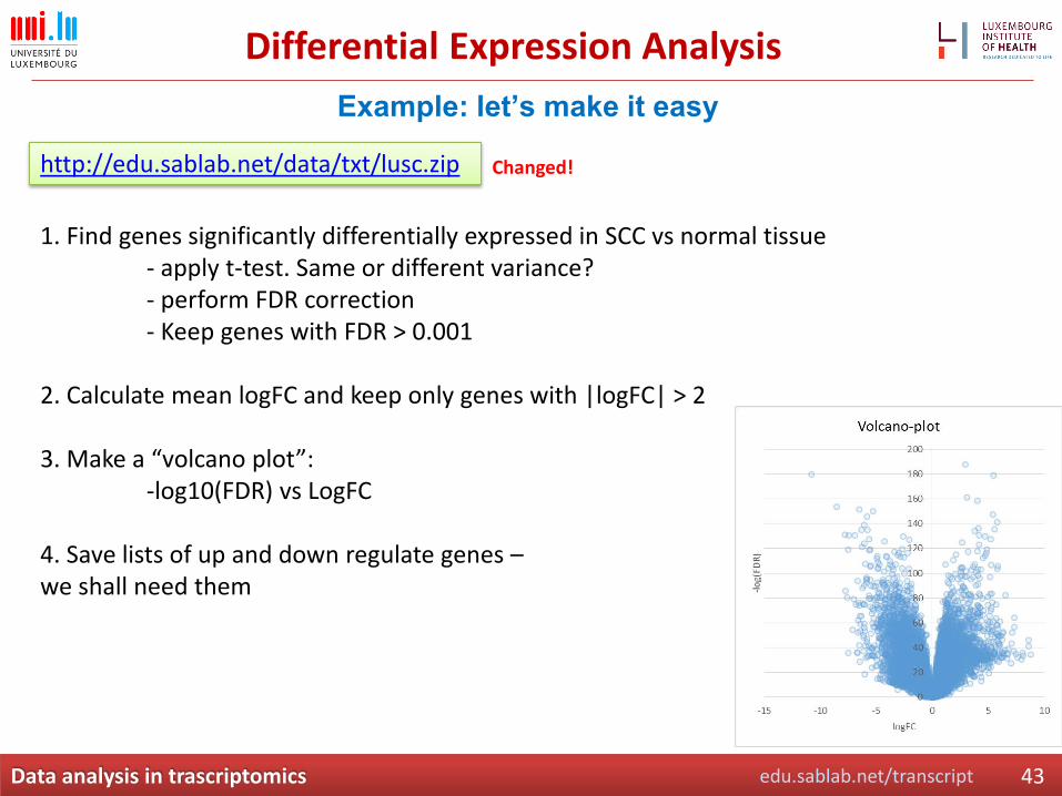
http://edu.sablab.net/data/txt/lusc.zip

1. Find genes significantly differentially expressed in SCC vs normal tissue - apply t-test. Same or different variance?- perform FDR correction- Keep genes with FDR > 0.001

2. Calculate mean logFC and keep only genes with |logFC| > 2

3. Make a “volcano plot”: -log10(FDR) vs LogFC

4. Save lists of up and down regulate genes –we shall need them

Example: let’s make it easy

Changed!



Classification


Classification and Marker Genes

Gene Markers

Questions

Based on which genes or gene sets we can predict the group of the samples?

How reliable is this prediction?



General Scheme

Experimental Data......................................................................................................................................................

Featureswith predictive power

110110001001001

110110

Analysis

Classification

001001001

0.0 0.2 0.4 0.6 0.8 1.0

0.0

0.2

0.4

0.6

0.8

1.0

(1-Specificity)

probability of false alarm

pro

ba

bility o

f d

ete

ctio

n(S

en

sitiv

ity)

ROC Curves

col 1 [ setosa vs. versicolor ]col 1 [ setosa vs. virginica ]col 1 [ versicolor vs. virginica ]

Confusion Matrix

A B C

pred.A 50 0 0

pred.B 0 48 2

pred.C 0 2 48



Selection of Features: Iris Dataset (Fisher)

Sepal.Length

2.0 3.0 4.0 0.5 1.5 2.5

4.5

6.5

2.0

3.5

Sepal.Width

Petal.Length

13

57

4.5 6.0 7.5

0.5

2.0

1 3 5 7

Petal.Width

4.5 5.0 5.5 6.0 6.5 7.0 7.5 8.0

0.0

0.4

0.8

1.2

Sepal.Length

N = 50 Bandwidth = 0.1229

Density

2.0 2.5 3.0 3.5 4.0

0.0

0.2

0.4

0.6

0.8

1.0

Sepal.Width


Density

1 2 3 4 5 6 7

0.0

0.5

1.0

1.5

2.0

2.5

Petal.Length

N = 50 Bandwidth = 0.05375

Density

0.5 1.0 1.5 2.0 2.5

02

46

Petal.Width

N = 50 Bandwidth = 0.03071

Density



Selection of Features: Iris Dataset

ROC curveis a graphical plot of the sensitivity, or true positive rate, vs. false positive rate (one minus the specificity or true negative rate)

4.5 5.0 5.5 6.0 6.5 7.0 7.5 8.0

0.0

0.4

0.8

1.2

Sepal.Length


Density

2.0 2.5 3.0 3.5 4.0

0.0

0.2

0.4

0.6

0.8

1.0

Sepal.Width


Density

1 2 3 4 5 6 7

0.0

0.5

1.0

1.5

2.0

2.5

Petal.Length

N = 50 Bandwidth = 0.05375

Density

0.5 1.0 1.5 2.0 2.5

02

46

Petal.Width

N = 50 Bandwidth = 0.03071

Density

AUCarea under ROC curve: 1 – ideal separation, 0.5 – random separation.



SVM Classification

Support vector machine (SVM) is a concept in statistics and computer science for a set of related supervised learning methods that analyze data and recognize patterns, used for classification and regression analysis.

library(e1071)

model = svm(Species ~ ., data = iris)

svm.res = as.character(predict(model, iris[,-5]))

## creat a confusion matrix

ConTab = data.frame(matrix(nr=3,nc=3))

rownames(ConTab) = paste("pred.",levels(iris$Species),sep="")

names(ConTab) = levels(iris$Species)

for (ic in 1:3){

for (ir in 1:3){

ConTab[ir,ic] = sum(iris$Species == levels(iris$Species)[ic] &

svm.res == levels(iris$Species)[ir])

}

}


Enrichment Analysis


Enrichment Analysis

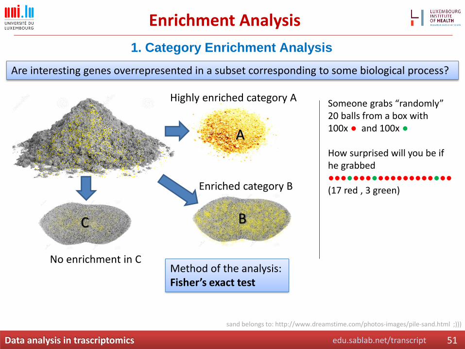
1. Category Enrichment Analysis

Are interesting genes overrepresented in a subset corresponding to some biological process?

Highly enriched category A

Enriched category B

No enrichment in C

sand belongs to: http://www.dreamstime.com/photos-images/pile-sand.html ;)))

Method of the analysis: Fisher’s exact test

A

BC

Someone grabs “randomly” 20 balls from a box with 100x ● and 100x ●

How surprised will you be if he grabbed ●●●●●●●●●●●●●●●●●●●●(17 red , 3 green)


Enrichment Analysis

1. Category Enrichment Analysis

Okamoto et al. Cancer Cell International 2007 7:11 doi:10.1186/1475-2867-7-11

Fisher’s exact test: based on hypergeometrical distributions

Hypergeometrical: distribution of objects taken from a “box”, without putting them back

𝐶𝑘𝑛 = 𝐶𝑛

𝑘 =𝑛𝑘

=𝑛!

𝑘! 𝑛 − 𝑘 !


Enrichment Analysis

2. Gene Set Enrichment Analysis (GSEA)

Is direction of genes in a category random?

A. Subramanian et al. PNAS 2005,102,43


Enrichment Analysis

Example: GO enrichment


Strategy 2:Separate DEG to down- and up- regulated genes. Then perform independent enrichment by these 2 groups

• Can be biased (gene can be ↑↓)• Assume ↑gene => ↑function• Can distinguish ↑ and ↓ functions

Strategy 1: Take all DEG and use them in enrichment.

• Safe• No additional assumptions• Cannot distinguish ↑ and ↓ functions

Enrichrhttp://amp.pharm.mssm.edu/Enrichr/enrich

BioCompendiumhttp://biocompendium.embl.de/


http://amp.pharm.mssm.edu/Enrichr/enrich

http://biocompendium.embl.de/


Enrichment Analysis


0. Prepare lists of DE genes…

1. Put up-regulated into enrich

3. Check: Down CMAP, Disease Signatures from GEO up,

4. Try biocompendium

5. Put top 100 genes into String to see PP-interactions

LUSC Example

Up regulated

Down regulated


http://string-db.org

http://amp.pharm.mssm.edu/Enrichr/



http://string-db.org/

http://amp.pharm.mssm.edu/Enrichr/


Summary

Raw Data

QA/QC+ Remove outliers

Normalization(remove technical artefacts,

make data comparable)

Visualization and exploratory analysis

(PCA, clustering)

Filtering(remove uninformative

features)

Processed Data

DEA(differential expression analysis)

Prediction(signatures for classification)

GSEA(gene set

enrichment analysis)

Enrichment(GO, functions,

TFs, drugs)

Network reconstruction

(not considered here)


Questions ?

Thank you for your attention !

Lecture 13 dr. P. Nazarov -...

Documents

Transcript of Lecture 13 dr. P. Nazarov -...