Lecture 13: Classification

6.0002 LECTURE 13 1

Announcements

Reading ◦ Chapter 24 ◦ Section 5.3.2 (list comprehension)

Course evaluations ◦ Online evaluation now through noon on Friday,

December 16

6.0002 LECTURE 13 2

Supervised Learning

Regression ◦ Predict a real number associated with a feature vector ◦ E.g., use linear regression to fit a curve to data

Classification ◦ Predict a discrete value (label) associated with a feature

vector

6.0002 LECTURE 13 3

An Example (similar to earlier lecture) Features Label

Name Egg-laying Scales Poisonous Cold-blooded

Number legs

Reptile

Cobra 1 1 1 1 0 1

Rattlesnake 1 1 1 1 0 1

Boa 0 1 0 1 0 1 constrictor

Chicken 1 1 0 1 2 0

Guppy 0 1 0 0 0 0

Dart frog 1 0 1 0 4 0

Zebra 0 0 0 0 4 0

Python 1 1 0 1 0 1

Alligator 1 1 0 1 4 1

6.0002 LECTURE 13 4

Distance Matrix

Code for producing this table posted

6.0002 LECTURE 13 5

Using Distance Matrix for Classification

Simplest approach is probably nearest neighbor Remember training data

When predicting the label of a new example ◦ Find the nearest example in the training data ◦ Predict the label associated with that example

X

6.0002 LECTURE 13 6

Distance Matrix

Label

R

R R

~R

~R

~R

6.0002 LECTURE 13 7

An Example

6.0002 LECTURE 13 8

K-nearest Neighbors

X

6.0002 LECTURE 13 9

An Example

6.0002 LECTURE 13 10

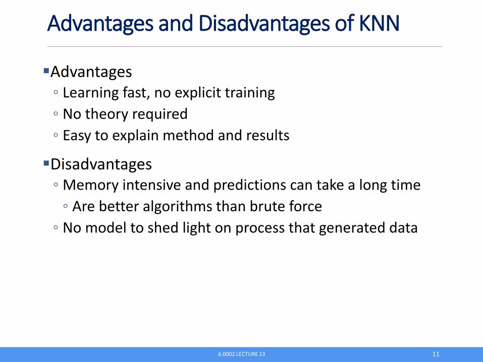
Advantages and Disadvantages of KNN

Advantages ◦ Learning fast, no explicit training ◦ No theory required ◦ Easy to explain method and results

Disadvantages ◦ Memory intensive and predictions can take a long time ◦ Are better algorithms than brute force ◦ No model to shed light on process that generated data

6.0002 LECTURE 13 11

The Titanic Disaster

RMS Titanic sank in the North Atlantic the morning of15 April 1912, after colliding with an iceberg. Of the 1,300 passengers aboard, 812 died. (703 of 918 crewmembers died.)

Database of 1046 passengers ◦ Cabin class ◦ 1st, 2nd, 3rd

◦ Age ◦ Gender

6.0002 LECTURE 13 12

Is Accuracy Enough

If we predict “died”, accuracy will be >62% orpassenger and >76% for crew members

Consider a disease that occurs in 0.1% of population ◦ Predicting disease-free has an accuracy of 0.999

6.0002 LECTURE 13 13

Other Metrics

sensitivity = recall specificity = precision

6.0002 LECTURE 13 14

Testing Methodology Matters

Leave-one-out

Repeated random subsampling

6.0002 LECTURE 13 15

Leave-one-out

6.0002 LECTURE 13 16

Repeated Random Subsampling

6.0002 LECTURE 13 17

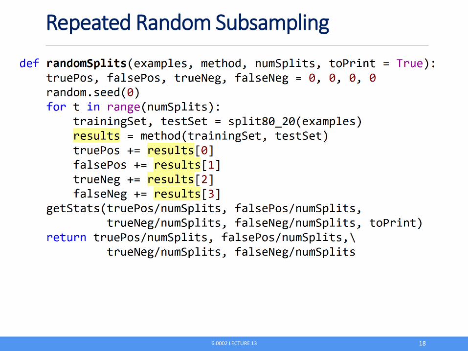
Repeated Random Subsampling

6.0002 LECTURE 13 18

Let’s Try KNN

6.0002 LECTURE 13 19

Results Average of 10 80/20 splits using KNN (k=3) Accuracy = 0.766 Sensitivity = 0.67 Specificity = 0.836 Pos. Pred. Val. = 0.747 Average of LOO testing using KNN (k=3) Accuracy = 0.769 Sensitivity = 0.663 Specificity = 0.842 Pos. Pred. Val. = 0.743

Considerably better than 62%

Not much difference between experiments

6.0002 LECTURE 13 20

Logistic Regression Analogous to linear regression

Designed explicitly for predicting probability of an event ◦ Dependent variable can only take on a finite set of values ◦ Usually 0 or 1

Finds weights for each feature ◦ Positive implies variable positively correlated with

outcome ◦ Negative implies variable negatively correlated with

outcome ◦ Absolute magnitude related to strength of the correlation

Optimization problem a bit complex, key is use of a logfunction—won’t make you look at it

6.0002 LECTURE 13 21

Class LogisticRegression

fit(sequence of feature vectors, sequence of labels) Returns object of type LogisticRegression

coef_ Returns weights of features

predict_proba(feature vector) Returns probabilities of labels

6.0002 LECTURE 13 22

Building a Model

6.0002 LECTURE 13 23

Applying Model

6.0002 LECTURE 13 24

List Comprehension

expr for id in L

Creates a list by evaluating expr len(L) times with id in expr replaced by each element of L

6.0002 LECTURE 13 25

Applying Model

6.0002 LECTURE 13 26

Putting It Together

6.0002 LECTURE 13 27

Results

Average of 10 80/20 splits LR Accuracy = 0.804 Sensitivity = 0.719 Specificity = 0.859 Pos. Pred. Val. = 0.767

Average of LOO testing using LR Accuracy = 0.786 Sensitivity = 0.705 Specificity = 0.842 Pos. Pred. Val. = 0.754

6.0002 LECTURE 13 28

Compare to KNN Results

Average of 10 80/20 splits using KNN (k=3) Accuracy = 0.744 Sensitivity = 0.629 Specificity = 0.829 Pos. Pred. Val. = 0.728

Average of LOO testing using KNN (k=3) Accuracy = 0.769 Sensitivity = 0.663 Specificity = 0.842 Pos. Pred. Val. = 0.743

Average of 10 80/20 splits LR Accuracy = 0.804 Sensitivity = 0.719 Specificity = 0.859 Pos. Pred. Val. = 0.767

Average of LOO testing using LR Accuracy = 0.786 Sensitivity = 0.705 Specificity = 0.842 Pos. Pred. Val. = 0.754

Performance not much difference Logistic regression slightly better

Also provides insight about variables

6.0002 LECTURE 13 29

Looking at Feature Weights

Be wary of reading too much into the weights Features are often correlated

model.classes_ = ['Died' 'Survived'] For label Survived

C1 = 1.66761946545 C2 = 0.460354552452 C3 = -0.50338282535 age = -0.0314481062387 male gender = -2.39514860929

6.0002 LECTURE 13 30

Changing the Cutoff

Try p = 0.1 Try p = 0.9 Accuracy = 0.493 Accuracy = 0.656 Sensitivity = 0.976 Sensitivity = 0.176 Specificity = 0.161 Specificity = 0.984 Pos. Pred. Val. = 0.444 Pos. Pred. Val. = 0.882

6.0002 LECTURE 13 31

ROC (Receiver Operating Characteristic)

6.0002 LECTURE 13 32

Output

6.0002 LECTURE 13 33

MIT OpenCourseWarehttps://ocw.mit.edu

6.0002 Introduction to Computational Thinking and Data ScienceFall 2016

For information about citing these materials or our Terms of Use, visit: https://ocw.mit.edu/terms.