Lecture 12-13

Angle Modulation

ELG3175 Introduction to Communication Systems

Introduction to Angle Modulation

•  In angle modulation, the amplitude of the modulated signal remains fixed while the information is carried by the angle of the carrier.

•  The process that transforms a message signal into an angle modulated signal is a nonlinear one.

•  This makes analysis of these signals more difficult. •  However, their modulation and demodulation are

rather simple to implement.

The angle of the carrier

•  Let θi(t) represent the instantaneous angle of the carrier.

•  We express an angle modulated signal by:

where Ac is the carrier amplitude.

( ))(cos)( tAts ic θ=

Instantaneous frequency

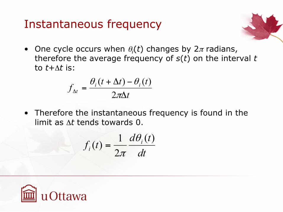
•  One cycle occurs when θi(t) changes by 2π radians, therefore the average frequency of s(t) on the interval t to t+Δt is:

•  Therefore the instantaneous frequency is found in the limit as Δt tends towards 0.

tttt

f iit Δ

−Δ+=Δ π

θθ2

)()(

dttd

tf ii

)(21)(

θπ

=

Phase modulation

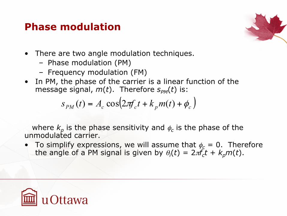
•  There are two angle modulation techniques. –  Phase modulation (PM) –  Frequency modulation (FM)

•  In PM, the phase of the carrier is a linear function of the message signal, m(t). Therefore sPM(t) is:

where kp is the phase sensitivity and φc is the phase of the unmodulated carrier. •  To simplify expressions, we will assume that φc = 0. Therefore

the angle of a PM signal is given by θi(t) = 2πfct + kpm(t).

( )cpccPM tmktfAts φπ ++= )(2cos)(

FM

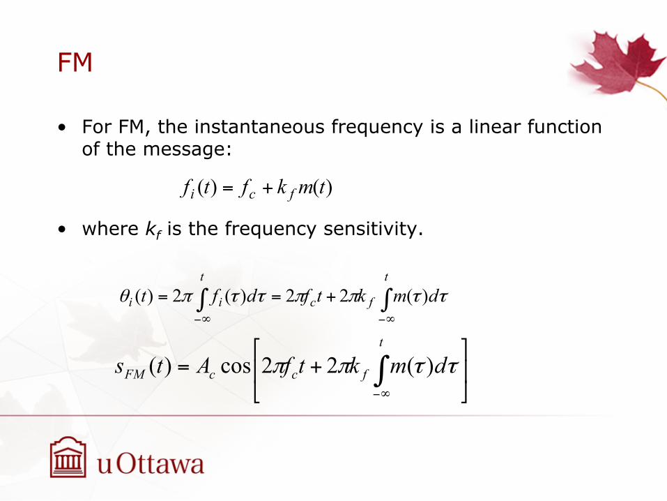
•  For FM, the instantaneous frequency is a linear function of the message:

•  where kf is the frequency sensitivity.

)()( tmkftf fci +=

∫∫∞−∞−

+==t

fc

t

ii dmktfdft ττππττπθ )(22)(2)(

⎥⎦

⎤⎢⎣

⎡+= ∫

∞−

t

fccFM dmktfAts ττππ )(22cos)(

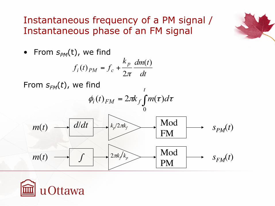
Instantaneous frequency of a PM signal / Instantaneous phase of an FM signal

•  From sPM(t), we find

From sFM(t), we find dttdmk

ftf pcPMi

)(2

)(π

+=

∫=t

fFMi dmkt0

)(2)( ττπφ

m(t) d/dt kp/2πkf Mod FM

sPM(t)

m(t) ∫ 2πkf/kp Mod PM

sFM(t)

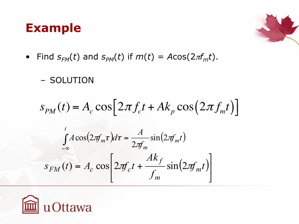
Example

•  Find sFM(t) and sPM(t) if m(t) = Acos(2πfmt).

–  SOLUTION

sPM (t) = Ac cos 2! fct + Akp cos 2! fmt( )!" #$

( ) ( )tffAdfA mm

t

m ππ

ττπ 2sin2

2cos =∫∞−

( )⎥⎦

⎤⎢⎣

⎡+= tffAk

tfAts mm

fccFM ππ 2sin2cos)(

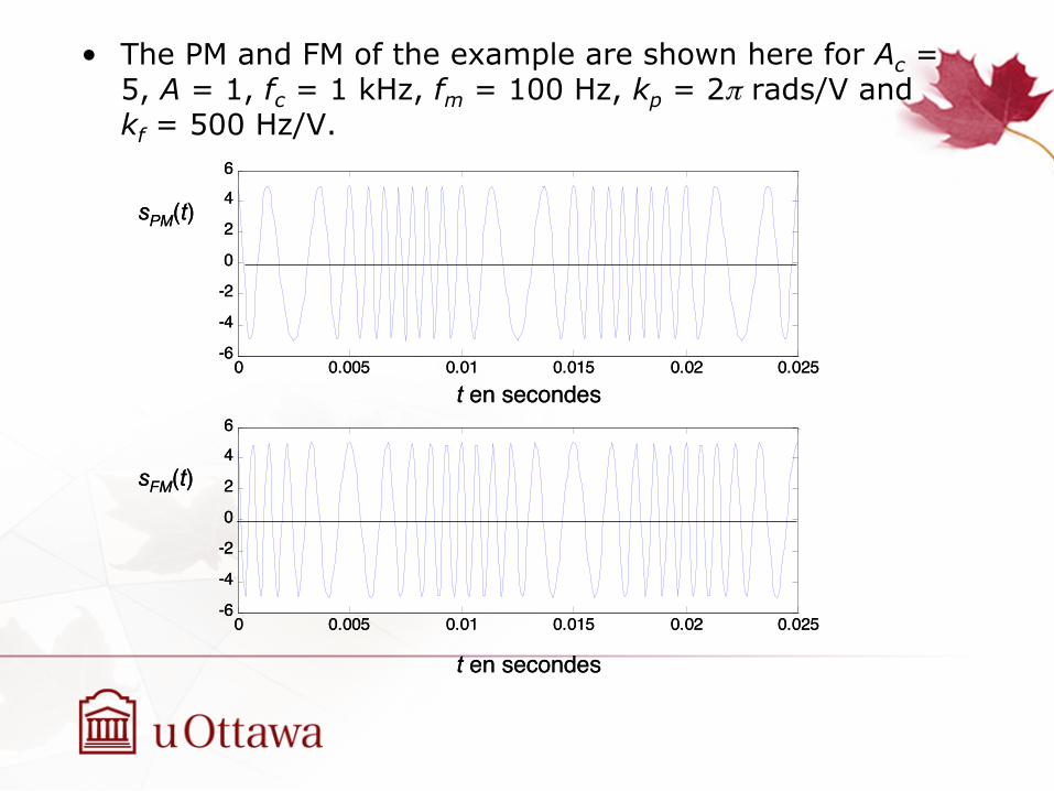
•  The PM and FM of the example are shown here for Ac = 5, A = 1, fc = 1 kHz, fm = 100 Hz, kp = 2π rads/V and kf = 500 Hz/V.

0 0.005 0.01 0.015 0.02 0.025-6

-4

-2

0

2

46

0 0.005 0.01 0.015 0.02 0.025-6

-4

-2

0

2

46

sPM(t)

sFM(t)

t en secondes

t en secondes

0 0.005 0.01 0.015 0.02 0.025-6

-4

-2

0

2

46

0 0.005 0.01 0.015 0.02 0.025-6

-4

-2

0

2

46

sPM(t)

sFM(t)

t en secondes

t en secondes

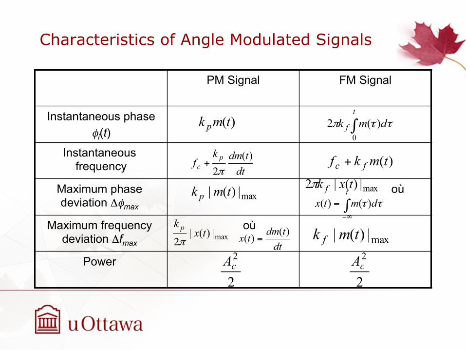
Characteristics of Angle Modulated Signals

PM Signal FM Signal

Instantaneous phase φi(t)

Instantaneous frequency

Maximum phase deviation Δφmax

où

Maximum frequency deviation Δfmax

où

Power

)(tmk p ∫t

f dmk0

)(2 ττπ

dttdmk

f pc

)(2π

+ )(tmkf fc +

max|)(| tmk p max|)(|2 txk fπ

∫∞−

=t

dmtx ττ )()(

max|)(|2tx

k pπ dt

tdmtx )()( = max|)(| tmk f

2

2cA

2

2cA

Modulation index

•  Assume that m(t) = Amcos(2πfmt). The resulting FM signals is:

•  For the FM signal

sFM (t) = Ac cos 2! fct +Amkffm

sin(2! fmt)!

"#

$

%&

mm

mfF f

ffAk maxΔ

==β

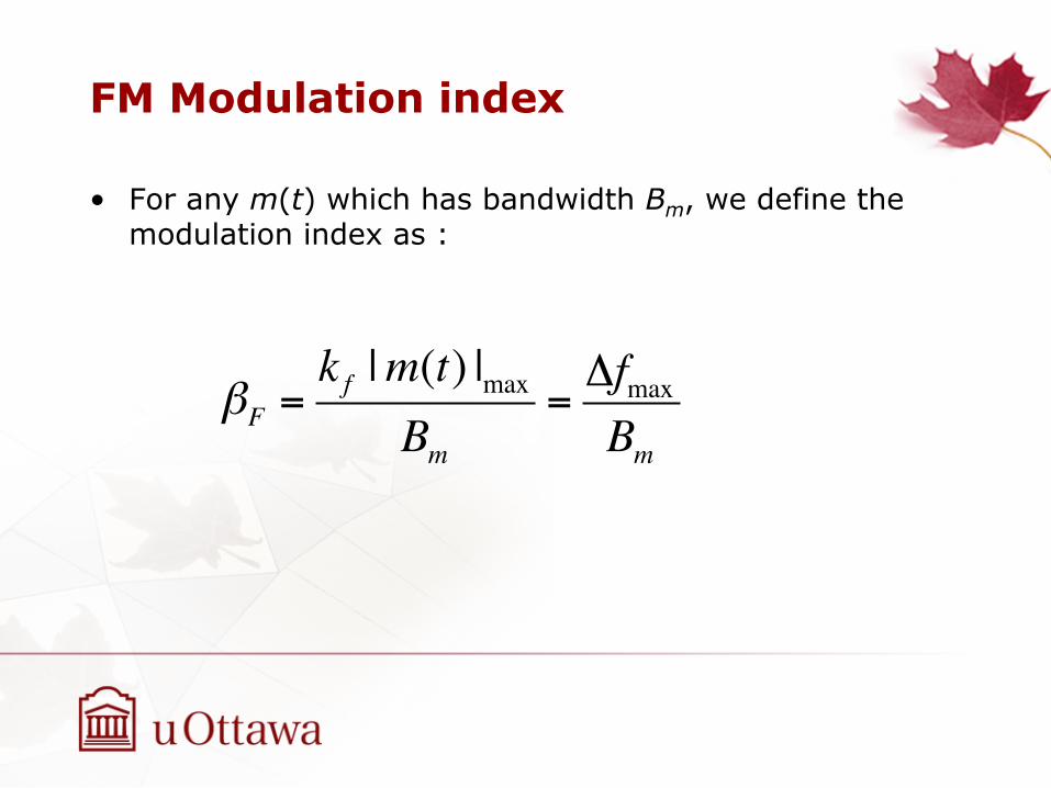
FM Modulation index

•  For any m(t) which has bandwidth Bm, we define the modulation index as :

!F =k f |m(t) |max

Bm=!fmaxBm

Example

•  The signal m(t) = 5sinc2(10t).

Find the modulation index for FM modulation with kf = 20 Hz/V.

–  SOLUTION

•  Bm = 10Hz, therefore βF = 20×5/10 = 10.

Narrowband FM

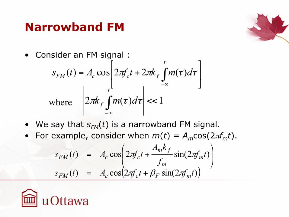
•  Consider an FM signal :

•  We say that sFM(t) is a narrowband FM signal. •  For example, consider when m(t) = Amcos(2πfmt).

⎥⎦

⎤⎢⎣

⎡+= ∫

∞−

t

fccFM dmktfAts ττππ )(22cos)(

1)(2 <<∫∞−

t

f dmk ττπwhere

( ))2sin(2cos)(

)2sin(2cos)(

tftfAts

tffkA

tfAts

mFccFM

mm

fmccFM

πβπ

ππ

+=

⎟⎟⎠

⎞⎜⎜⎝

⎛+=

Narrowband FM

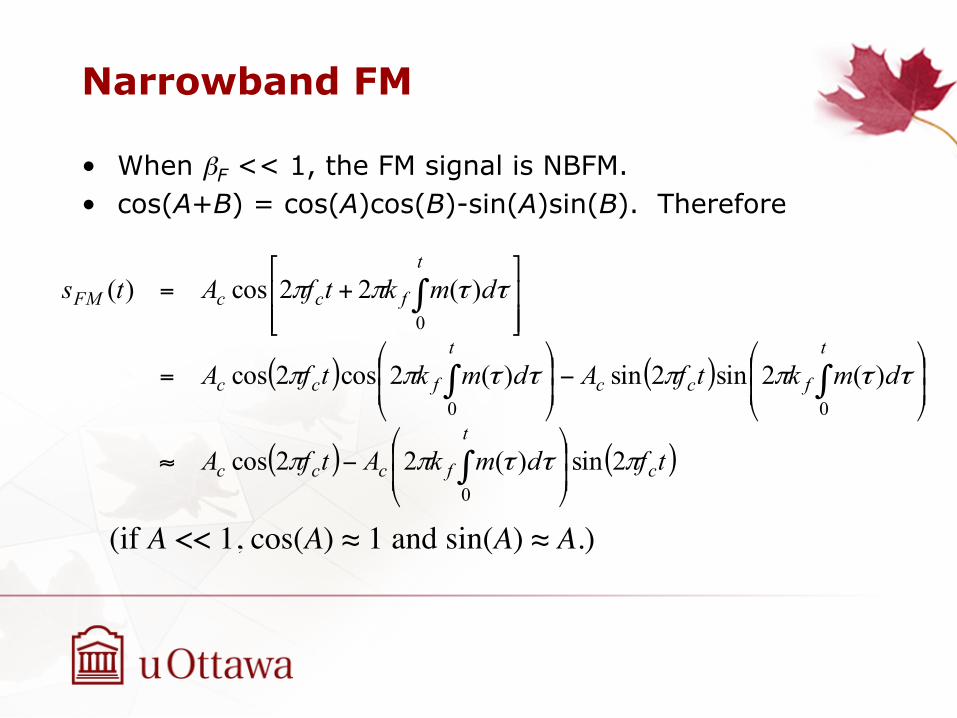
•  When βF << 1, the FM signal is NBFM. •  cos(A+B) = cos(A)cos(B)-sin(A)sin(B). Therefore

( ) ( )

( ) ( )tfdmkAtfA

dmktfAdmktfA

dmktfAts

c

t

fccc

t

fcc

t

fcc

t

fccFM

πττππ

ττππττππ

ττππ

2sin)(22cos

)(2sin2sin)(2cos2cos

)(22cos)(

0

00

0

⎟⎟⎠

⎞⎜⎜⎝

⎛−≈

⎟⎟⎠

⎞⎜⎜⎝

⎛−⎟⎟⎠

⎞⎜⎜⎝

⎛=

⎥⎥⎦

⎤

⎢⎢⎣

⎡+=

∫

∫∫

∫

(if A << 1, cos(A) ≈ 1 and sin(A) ≈ A.)

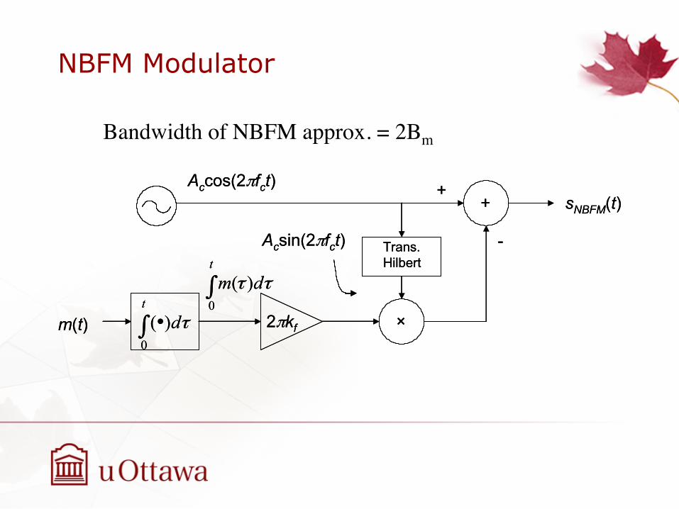
NBFM Modulator

Accos(2πfct)

m(t) ∫ •t

d0)( τ

∫t

dm0

)( ττ

2πkf ×

Trans. Hilbert

++

-

sNBFM(t)

Acsin(2πfct)

Accos(2πfct)

m(t) ∫ •t

d0)( τ

∫t

dm0

)( ττ

2πkf ×

Trans. Hilbert

++

-

sNBFM(t)

Acsin(2πfct)

Bandwidth of NBFM approx. = 2Bm

Wideband FM - WBFM

•  For an FM signal to be NBFM, βF << 1. •  Any signal that is not narrowband is therefore

wideband. •  However, typically βF > 1 for an FM signal to be

considered wideband. •  The bandwidth of WBFM signals is larger than NBFM

since Δfmax is increased.

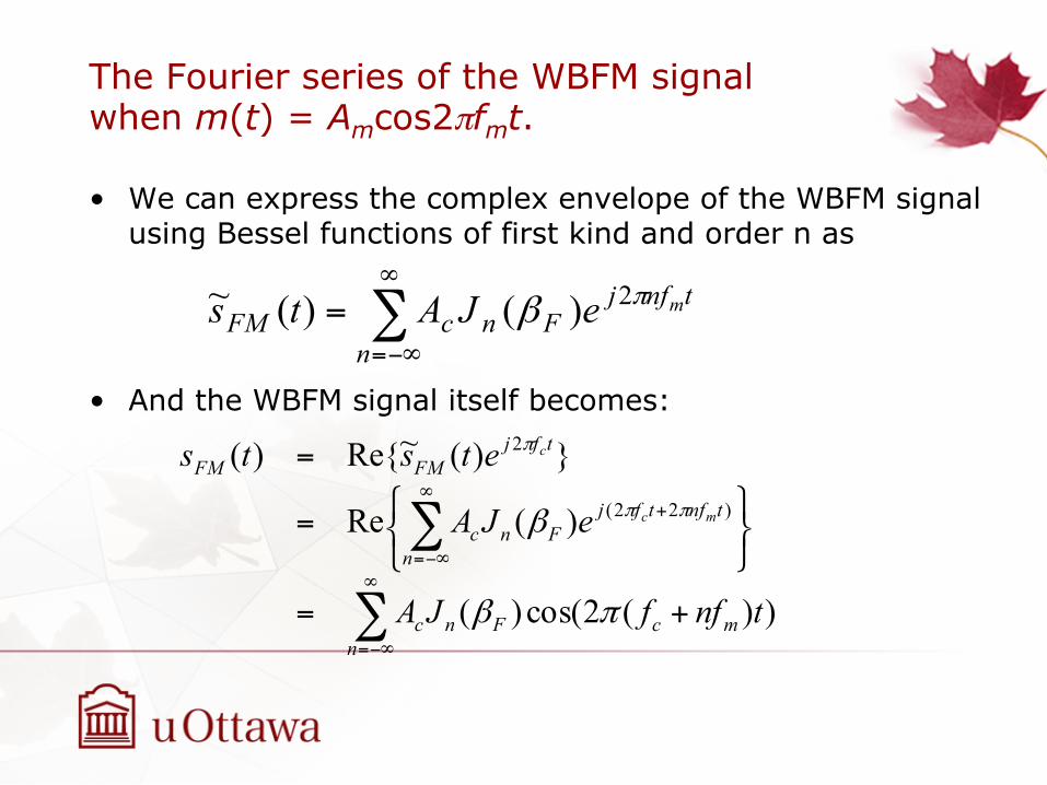
The Fourier series of the WBFM signal when m(t) = Amcos2πfmt.

•  We can express the complex envelope of the WBFM signal using Bessel functions of first kind and order n as

•  And the WBFM signal itself becomes:

∑∞

−∞=

=n

tnfjFncFM

meJAts πβ 2)()(~

∑

∑∞

−∞=

∞

−∞=

+

+=

⎭⎬⎫

⎩⎨⎧

=

=

nmcFnc

n

tnftfjFnc

tfjFMFM

tnffJA

eJA

etstsmc

c

))(2cos()(

)(Re

})(~Re{)()22(

2

πβ

β ππ

π

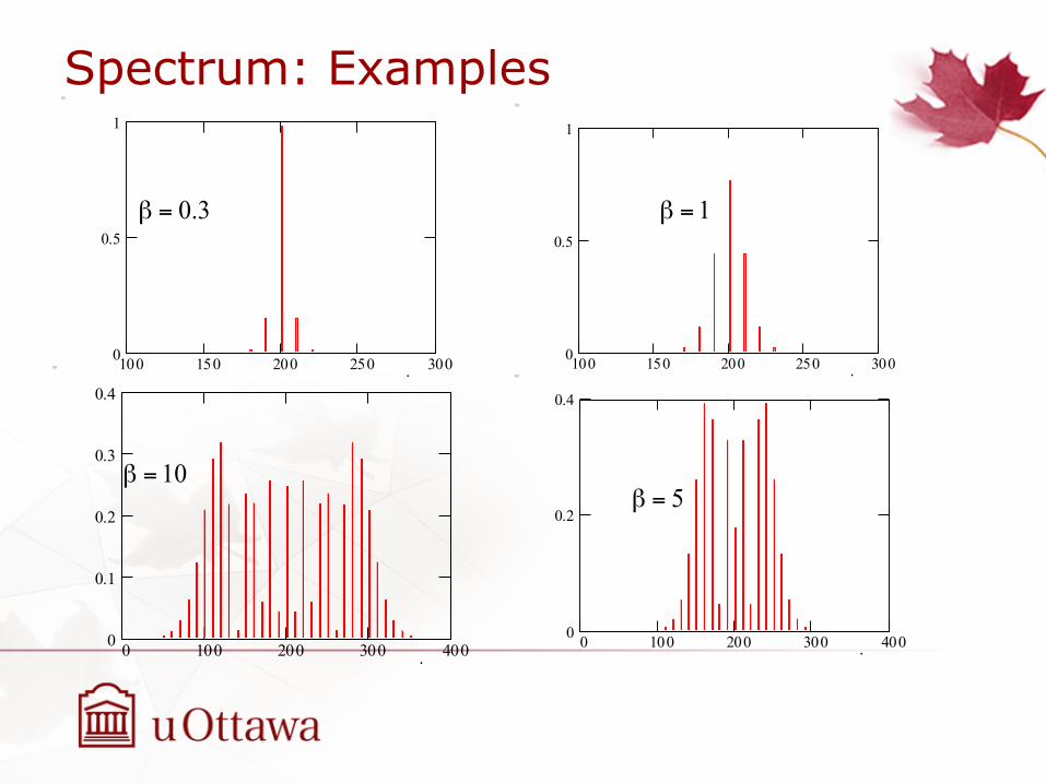
Spectrum: Examples

100 150 200 250 3000

0.5

1

.

0.3β =

100 150 200 250 3000

0.5

1

.

1β =

5β =

0 100 200 300 4000

0.1

0.2

0.3

0.4

.0 100 200 300 4000

0.2

0.4

.

10β =

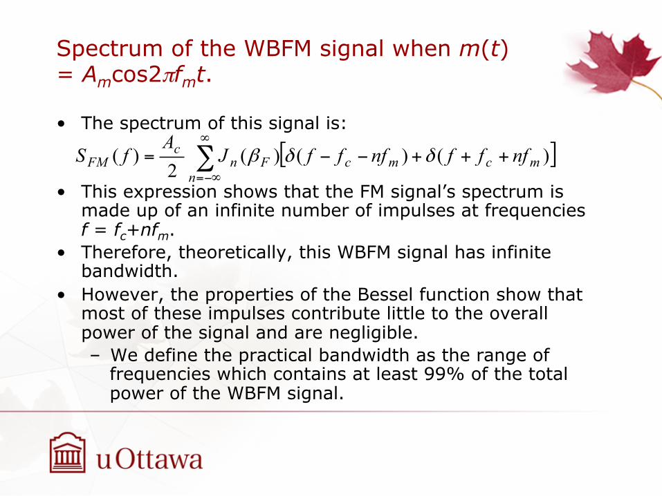
Spectrum of the WBFM signal when m(t) = Amcos2πfmt.

•  The spectrum of this signal is:

•  This expression shows that the FM signal’s spectrum is

made up of an infinite number of impulses at frequencies f = fc+nfm.

•  Therefore, theoretically, this WBFM signal has infinite bandwidth.

•  However, the properties of the Bessel function show that most of these impulses contribute little to the overall power of the signal and are negligible. –  We define the practical bandwidth as the range of

frequencies which contains at least 99% of the total power of the WBFM signal.

[ ]∑∞

−∞=

+++−−=n

mcmcFnc

FM nfffnfffJA

fS )()()(2

)( δδβ

Lecture 6

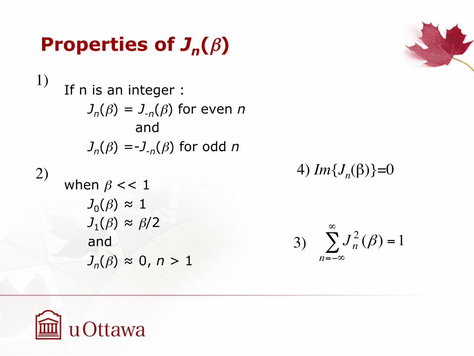
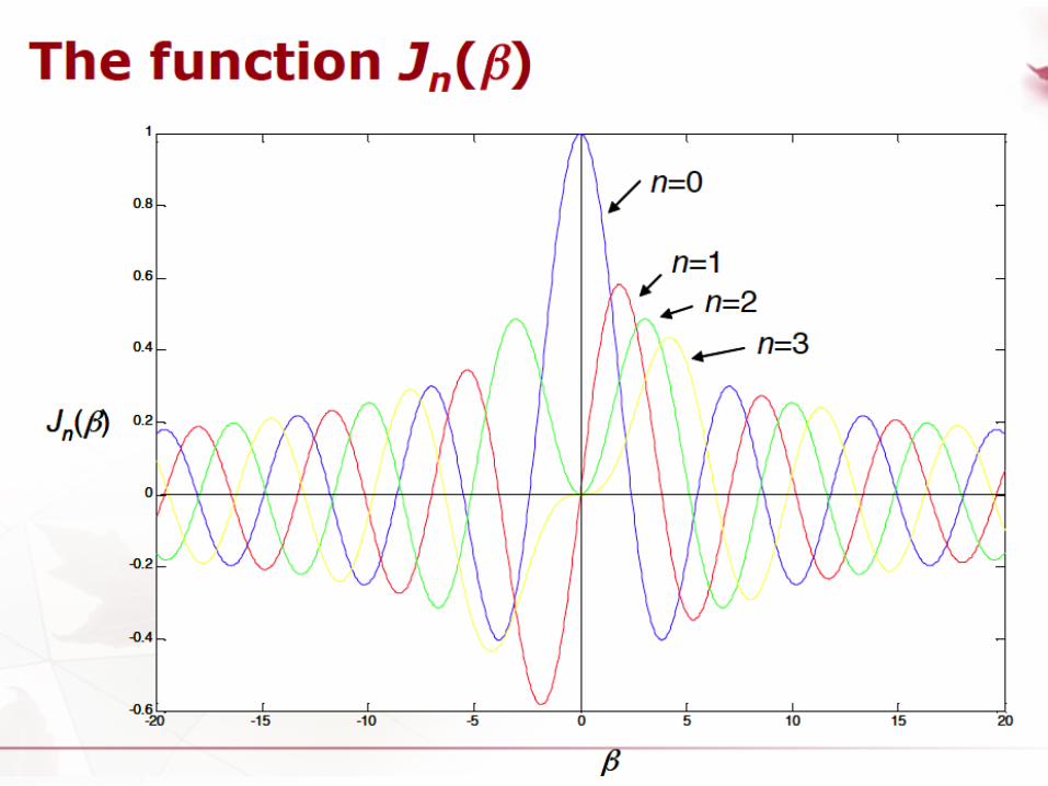
Properties of Jn(β)

If n is an integer : Jn(β) = J-n(β) for even n and Jn(β) =-J-n(β) for odd n when β << 1

J0(β) ≈ 1 J1(β) ≈ β/2 and Jn(β) ≈ 0, n > 1

∑∞

−∞=

=n

nJ 1)(2 β

1)

2)

3)

4) Im{Jn(β)}=0

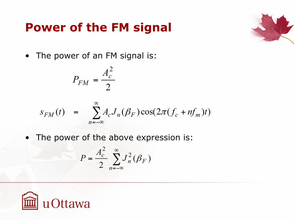
Power of the FM signal

•  The power of an FM signal is:

•  The power of the above expression is:

2

2c

FMA

P =

∑∞

−∞=

+=n

mcFncFM tnffJAts ))(2cos()()( πβ

∑∞

−∞=

=n

Fnc JA

P )(2

22

β

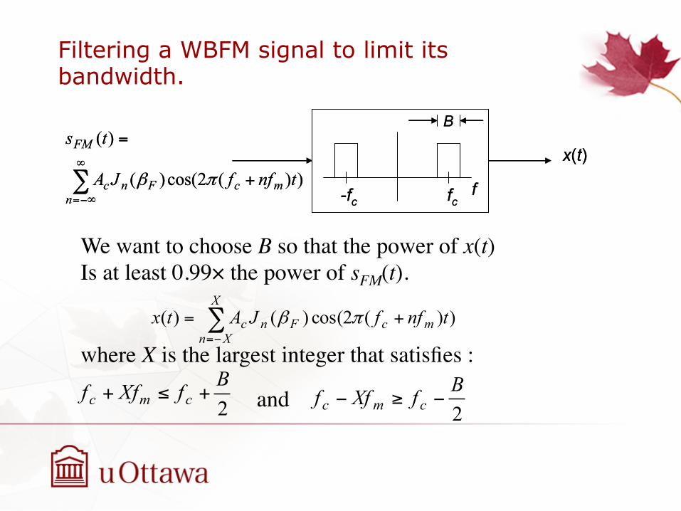
Filtering a WBFM signal to limit its bandwidth.

B

f

x(t)∑∞

−∞=

+

=

nmcFnc

FM

tnffJA

ts

))(2cos()(

)(

πβ-fc fc

B

f

x(t)∑∞

−∞=

+

=

nmcFnc

FM

tnffJA

ts

))(2cos()(

)(

πβ-fc fc

We want to choose B so that the power of x(t) Is at least 0.99× the power of sFM(t). where X is the largest integer that satisfies :

∑−=

+=X

XnmcFnc tnffJAtx ))(2cos()()( πβ

2BfXff cmc +≤+ and

2BfXff cmc −≥−

•  The power of x(t) is:

•  Therefore we must choose X so that:

•  We know that Jn2(βF) = J-n

2(βF). Therefore

∑−=

=X

XnFn

cx JAP )(

22

2

β

99.0)(2 ≥∑−=

X

XnFnJ β

99.0)(2)(1

220 ≥+ ∑

=

X

nFnF JJ ββ

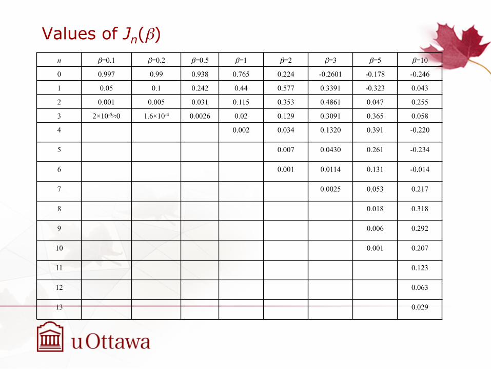
Values of Jn(β) n β=0.1 β=0.2 β=0.5 β=1 β=2 β=3 β=5 β=10 0 0.997 0.99 0.938 0.765 0.224 -0.2601 -0.178 -0.246 1 0.05 0.1 0.242 0.44 0.577 0.3391 -0.323 0.043 2 0.001 0.005 0.031 0.115 0.353 0.4861 0.047 0.255 3 2×10-5≈0 1.6×10-4 0.0026 0.02 0.129 0.3091 0.365 0.058 4 0.002 0.034 0.1320 0.391 -0.220 5 0.007 0.0430 0.261 -0.234 6 0.001 0.0114 0.131 -0.014 7 0.0025 0.053 0.217 8 0.018 0.318 9 0.006 0.292 10 0.001 0.207 11 0.123 12 0.063 13 0.029

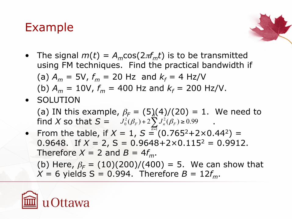
Example

•  The signal m(t) = Amcos(2πfmt) is to be transmitted using FM techniques. Find the practical bandwidth if (a) Am = 5V, fm = 20 Hz and kf = 4 Hz/V (b) Am = 10V, fm = 400 Hz and kf = 200 Hz/V.

•  SOLUTION (a) IN this example, βF = (5)(4)/(20) = 1. We need to find X so that S = .

•  From the table, if X = 1, S = (0.7652+2×0.442) = 0.9648. If X = 2, S = 0.9648+2×0.1152 = 0.9912. Therefore X = 2 and B = 4fm. (b) Here, βF = (10)(200)/(400) = 5. We can show that X = 6 yields S = 0.994. Therefore B = 12fm.

99.0)(2)(1

220 ≥+ ∑

=

X

nFnF JJ ββ

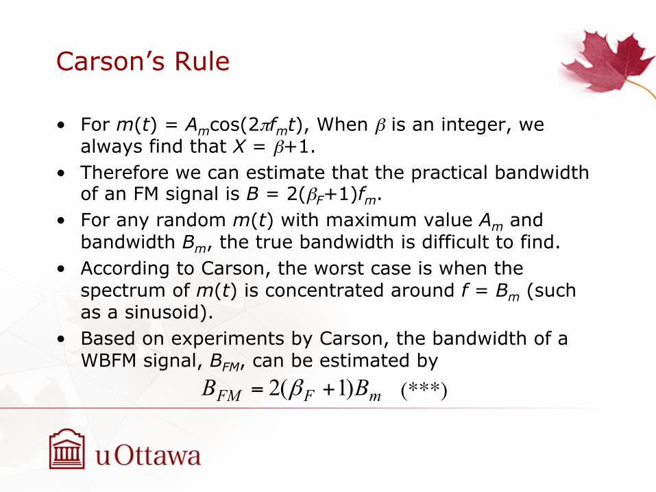
Carson’s Rule

•  For m(t) = Amcos(2πfmt), When β is an integer, we always find that X = β+1.

•  Therefore we can estimate that the practical bandwidth of an FM signal is B = 2(βF+1)fm.

•  For any random m(t) with maximum value Am and bandwidth Bm, the true bandwidth is difficult to find.

•  According to Carson, the worst case is when the spectrum of m(t) is concentrated around f = Bm (such as a sinusoid).

•  Based on experiments by Carson, the bandwidth of a WBFM signal, BFM, can be estimated by

mFFM BB )1(2 += β (***)

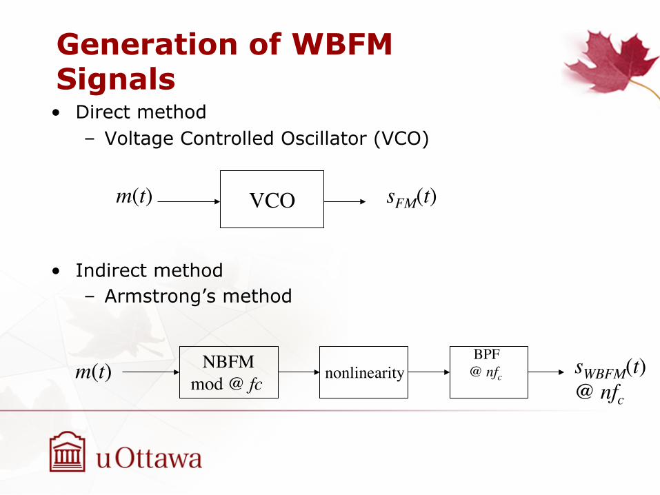
Generation of WBFM Signals •  Direct method

–  Voltage Controlled Oscillator (VCO)

•  Indirect method –  Armstrong’s method

m(t) VCO sFM(t)

m(t) NBFM mod @ fc nonlinearity

BPF @ nfc sWBFM(t)

@ nfc

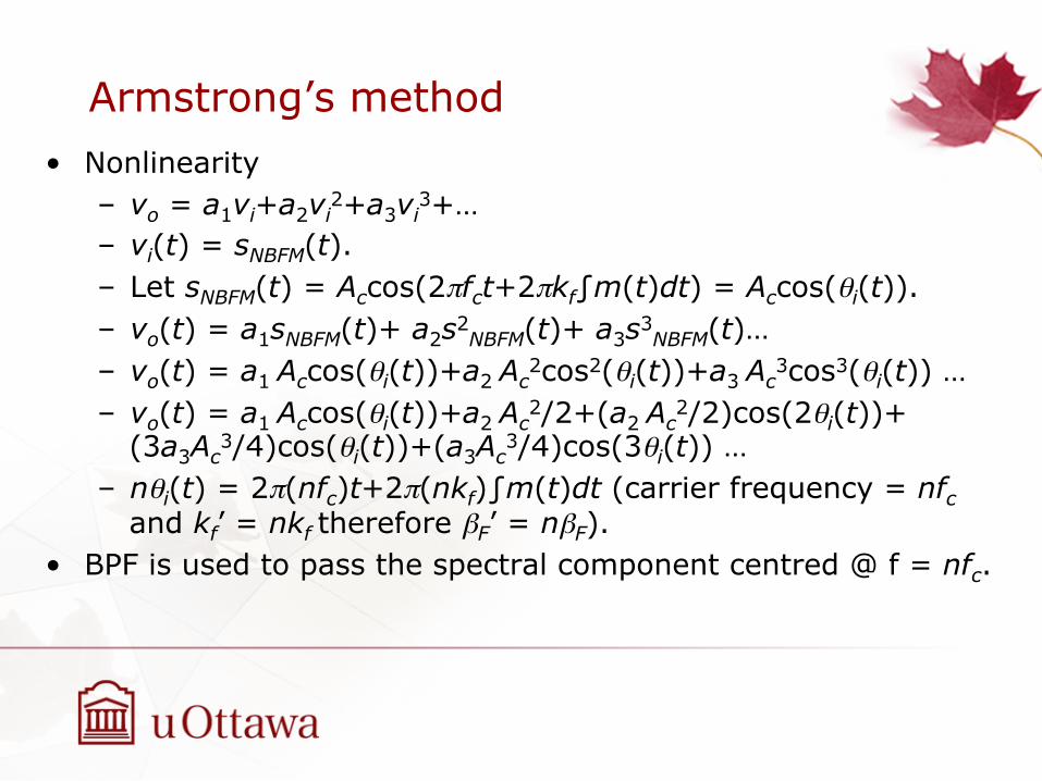
Armstrong’s method •  Nonlinearity

–  vo = a1vi+a2vi2+a3vi

3+… –  vi(t) = sNBFM(t). –  Let sNBFM(t) = Accos(2πfct+2πkf∫m(t)dt) = Accos(θi(t)). –  vo(t) = a1sNBFM(t)+ a2s2

NBFM(t)+ a3s3NBFM(t)…

–  vo(t) = a1 Accos(θi(t))+a2 Ac2cos2(θi(t))+a3 Ac

3cos3(θi(t)) … –  vo(t) = a1 Accos(θi(t))+a2 Ac

2/2+(a2 Ac2/2)cos(2θi(t))+

(3a3Ac3/4)cos(θi(t))+(a3Ac

3/4)cos(3θi(t)) … –  nθi(t) = 2π(nfc)t+2π(nkf)∫m(t)dt (carrier frequency = nfc

and kf’ = nkf therefore βF’ = nβF). •  BPF is used to pass the spectral component centred @ f = nfc.

Demodulation of FM signals

•  Differentiator plus envelope detection •  Frequency discriminator. •  Frequency counter.

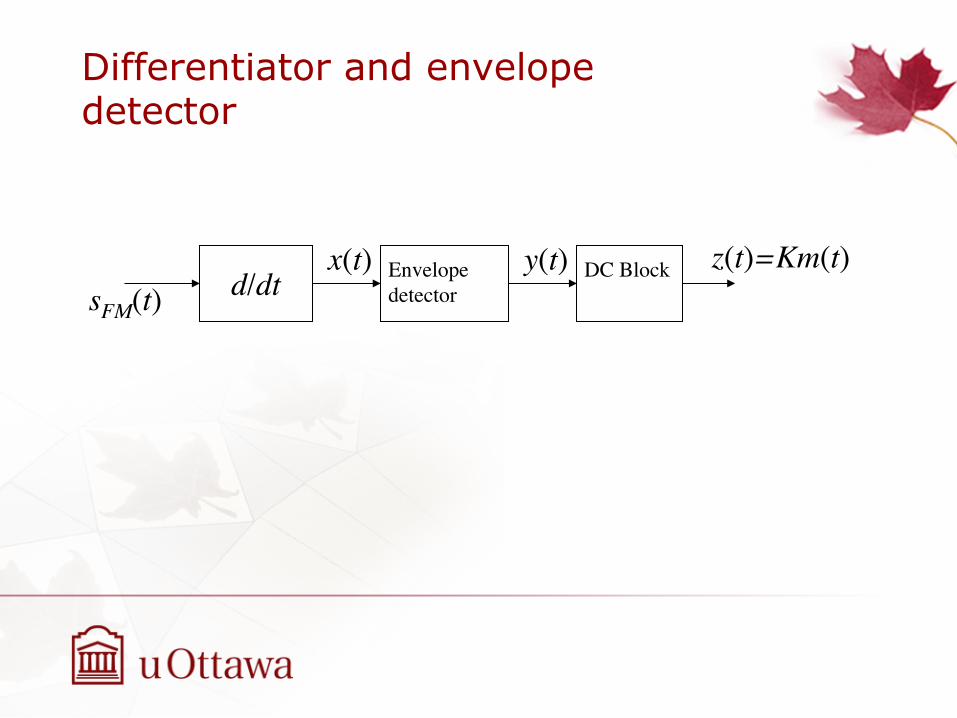
Differentiator and envelope detector

sFM(t) d/dt x(t) Envelope

detector DC Block y(t) z(t)=Km(t)

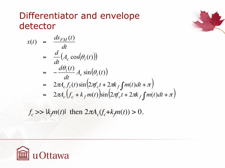
Differentiator and envelope detector

( )( )

( )( )

( ) ( )ππππ

ππππ

θθ

θ

+++=

++=

−=

=

=

∫∫

dttmktftmkfAdttmktftfA

tAdttd

tAdtddttdstx

fcfcc

fcic

ici

ic

FM

)(22sin)(2)(22sin)(2

)(sin)(

)(cos

)()(

fc >> |kfm(t)| then 2πAc(fc+kfm(t)) > 0.

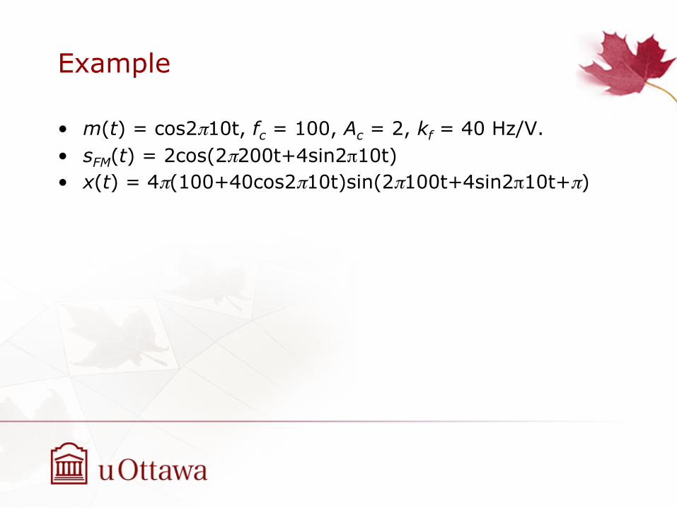
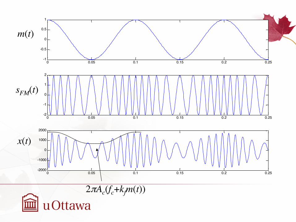
Example

•  m(t) = cos2π10t, fc = 100, Ac = 2, kf = 40 Hz/V. •  sFM(t) = 2cos(2π200t+4sin2π10t) •  x(t) = 4π(100+40cos2π10t)sin(2π100t+4sin2π10t+π)

0 0.05 0.1 0.15 0.2 0.25-1

-0.5

0

0.5

1

0 0.05 0.1 0.15 0.2 0.25-2

-1

0

1

2

0 0.05 0.1 0.15 0.2 0.25-2000

-1000

0

1000

2000

m(t)

sFM(t)

x(t)

2πAc(fc+kfm(t))

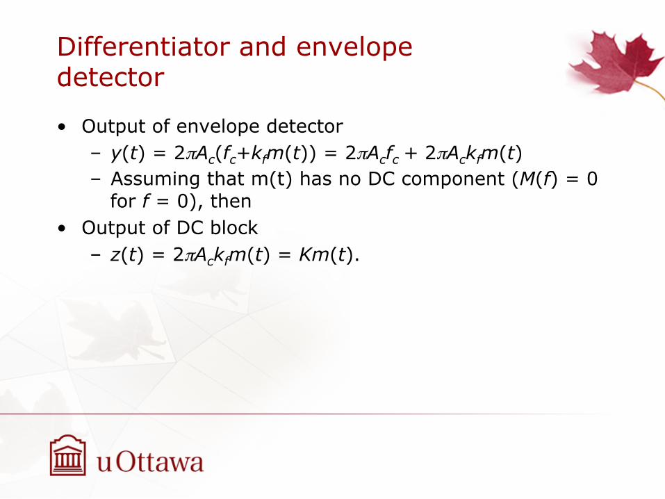
Differentiator and envelope detector

•  Output of envelope detector –  y(t) = 2πAc(fc+kfm(t)) = 2πAcfc + 2πAckfm(t) –  Assuming that m(t) has no DC component (M(f) = 0

for f = 0), then •  Output of DC block

–  z(t) = 2πAckfm(t) = Km(t).

Frequency discriminator

•  Similar to differentiator •  Input to envelope detector has lower amplitude.

sFM(t)

H1(f)

H2(f)

E.D

E.D

+ +

-

x1(t)

x2(t)

y1(t)

y2(t)

Km(t)

3-Jun-13

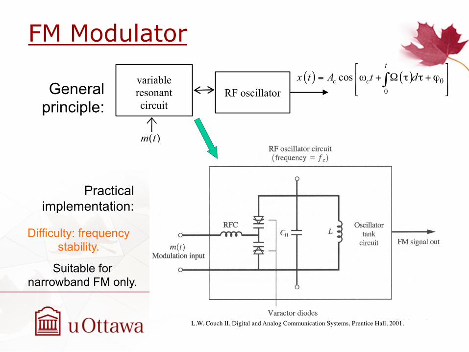
FM Modulator

RF oscillator

( )m t

( ) ( ) 00

cost

c cx t A t d⎡ ⎤

= ω + Ω τ τ + ϕ⎢ ⎥⎢ ⎥⎣ ⎦

∫variable resonant circuit

General principle:

Practical implementation:

Difficulty: frequency stability.

Suitable for narrowband FM only.

L.W. Couch II, Digital and Analog Communication Systems, Prentice Hall, 2001.

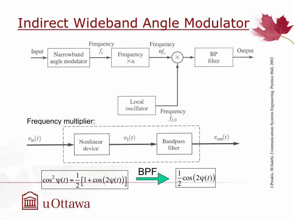
Indirect Wideband Angle Modulator

Frequency multiplier:

( )2 1cos ( ) 1 cos 2 ( )2

t tψ = + ψ⎡ ⎤⎣ ⎦ ( )1 cos 2 ( )2

tψBPF

J.Pro

akis,

M.S

aleh

i, Co

mm

unic

atio

ns S

yste

ms E

ngin

eerin

g, P

rent

ice

Hal

l, 20

02

Direct Wideband Angle Modulator

L.W. Couch II, Digital and Analog Communication Systems, Prentice Hall, 2001.

how it operates? consider it without feedback first why is feedback required? why is frequency divider required?

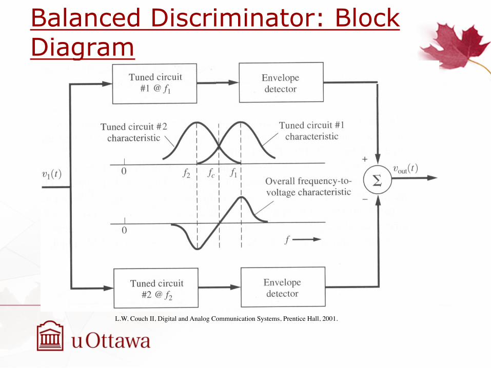
Balanced Discriminator: Block Diagram

L.W. Couch II, Digital and Analog Communication Systems, Prentice Hall, 2001.

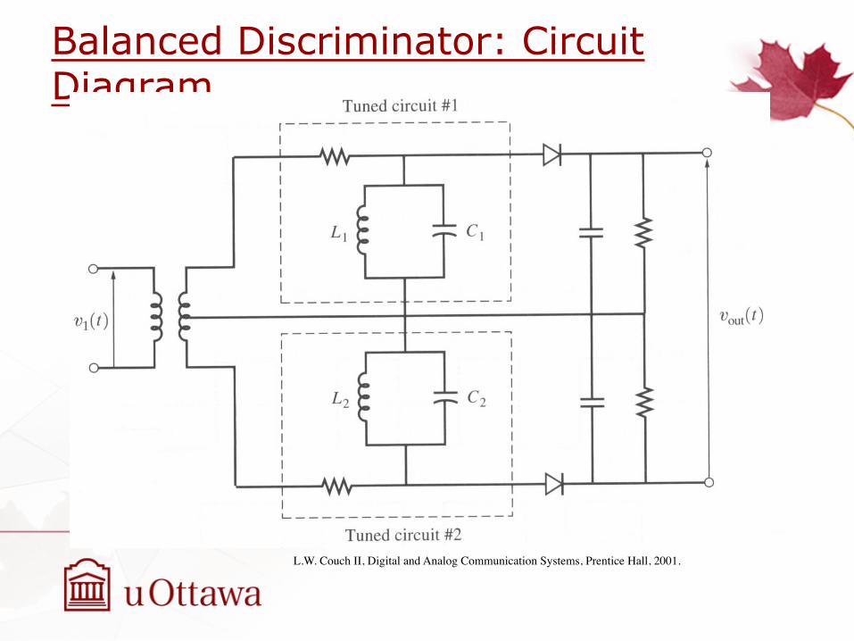
Balanced Discriminator: Circuit Diagram

L.W. Couch II, Digital and Analog Communication Systems, Prentice Hall, 2001.

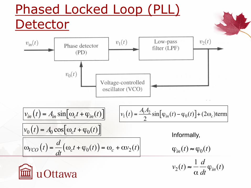
Phased Locked Loop (PLL) Detector

( ) [ ]sin ( )in in c inv t A t t= ω +ϕ

( ) [ ]0 0 0cos ( )cv t A t t= ω +ϕ

( ) ( )0 2( ) ( )VCO c cdt t t v tdt

ω = ω +ϕ = ω +α

Informally,

0( ) ( )in t tϕ ≈ ϕ

21( ) ( )indv t tdt

≈ ϕα

( ) [ ]1 21 0sin ( ) ( ) (2 )term

2 in cA Av t t t= ϕ −ϕ + ω

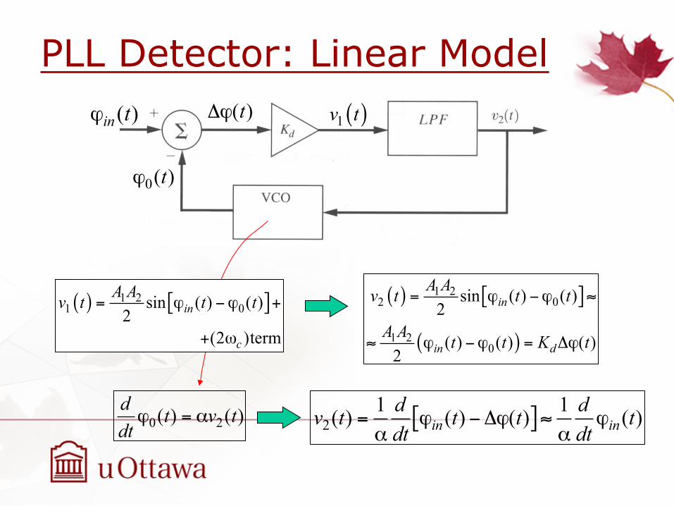
PLL Detector: Linear Model ( )in tϕ

0( )tϕ

( )tΔϕ ( )1v t

0 2( ) ( )d t v tdtϕ = α

( ) [ ]

( )

1 22 0

1 20

sin ( ) ( )2

( ) ( ) ( )2

in

in d

A Av t t t

A A t t K t

= ϕ −ϕ ≈

≈ ϕ −ϕ = Δϕ

[ ]21 1( ) ( ) ( ) ( )in ind dv t t t tdt dt

= ϕ − Δϕ ≈ ϕα α

( ) [ ]1 21 0sin ( ) ( )

2(2 )term

in

c

A Av t t t= ϕ − ϕ +

+ ω

Comparison of AM and FM/PM •  AM is simple (envelope detector) but no noise/

interference immunity (low quality). •  AM bandwidth is twice or the same as the

modulating signal (no bandwidth expansion). •  Power efficiency is low for conventional AM. •  DSB-SC & SSB – good power efficiency, but

complex circuitry. •  FM/PM – spectrum expansion & noise immunity.

Good quality. •  More complex circuitry. However, ICs allow for

cost-effective implementation.

Important Properties of Angle-Modulated Signals: Summary •  FM/PM signal is a nonlinear function of the

message. •  The signal’s bandwidth increases with the

modulation index. •  The carrier spectral level varies with the

modulation index, being 0 in some cases. •  Narrowband FM/PM: the signal’s bandwidth is

twice that of the message (the same as for AM). •  The amplitude of the FM/PM signal is constant

(hence, the power does not depend on the message).