Lecture 11

Comparing Two Means

Two Sample Problems:

The goal of inference is to compare the responses in two groups.

Each group is considered to be a sample from a distinct population.

The responses in each group are independent of those in the other group.

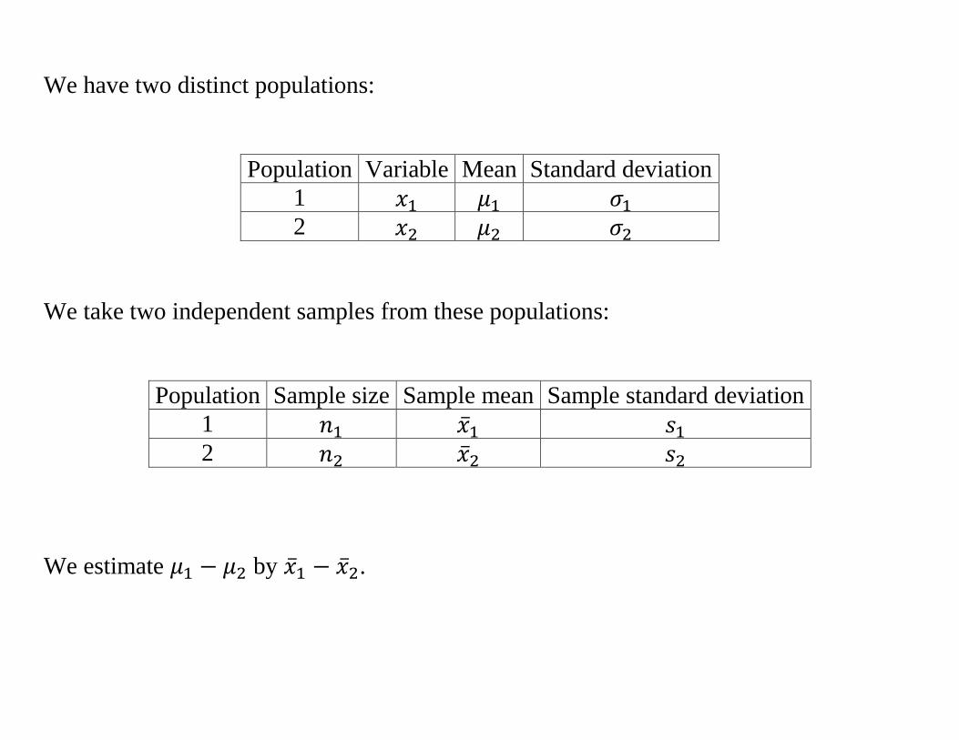
We have two distinct populations:

Population Variable Mean Standard deviation

1

2

We take two independent samples from these populations:

Population Sample size Sample mean Sample standard deviation

1

2

We estimate by .

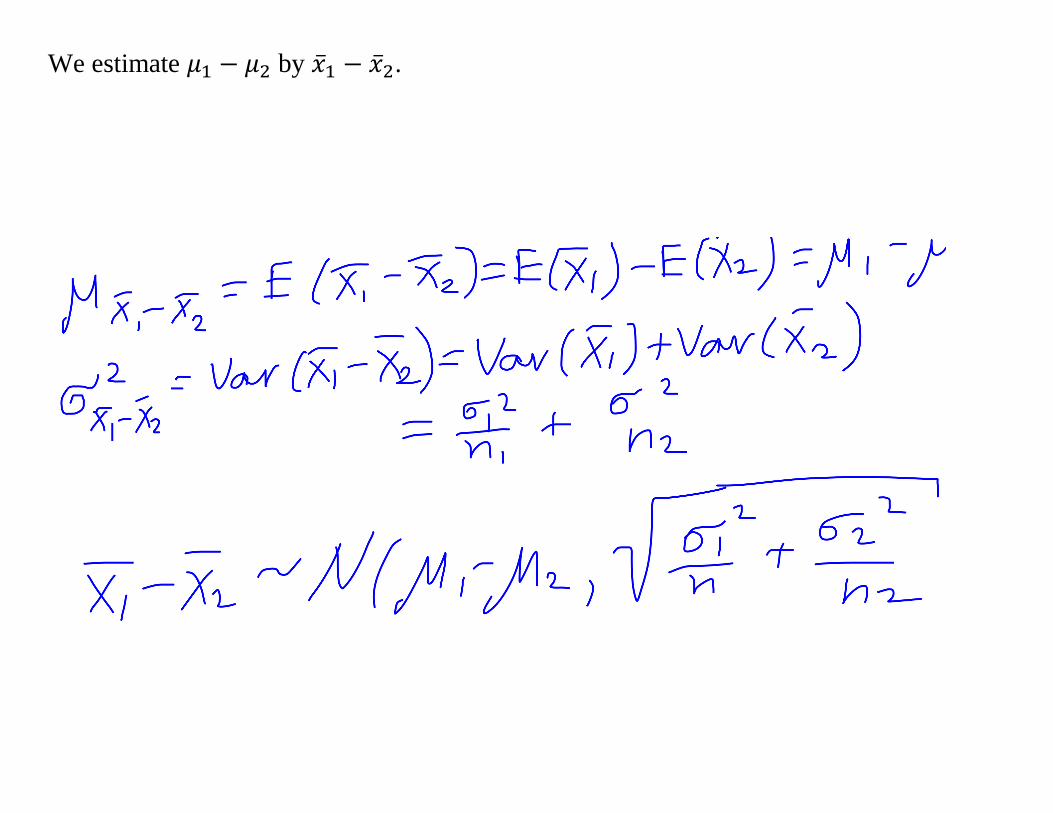
We estimate by .

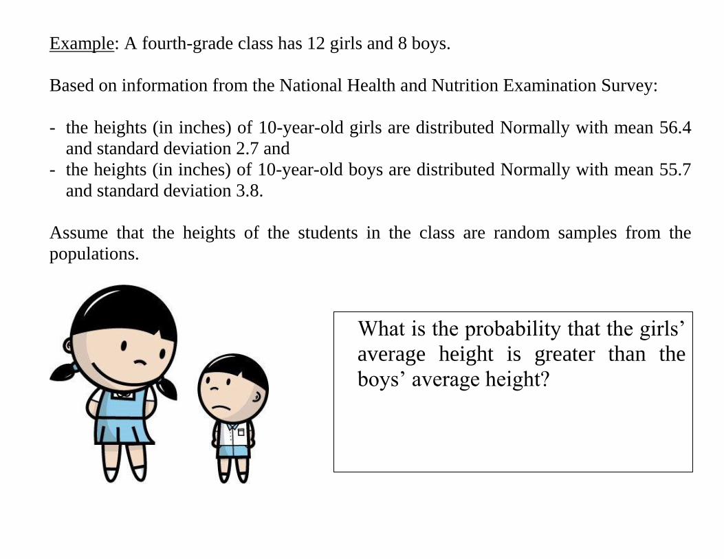
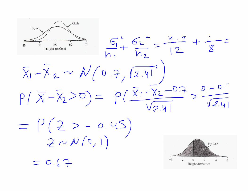
Example: A fourth-grade class has 12 girls and 8 boys.

Based on information from the National Health and Nutrition Examination Survey:

- the heights (in inches) of 10-year-old girls are distributed Normally with mean 56.4

and standard deviation 2.7 and

- the heights (in inches) of 10-year-old boys are distributed Normally with mean 55.7

and standard deviation 3.8.

Assume that the heights of the students in the class are random samples from the

populations.

What is the probability that the girls’

average height is greater than the

boys’ average height?

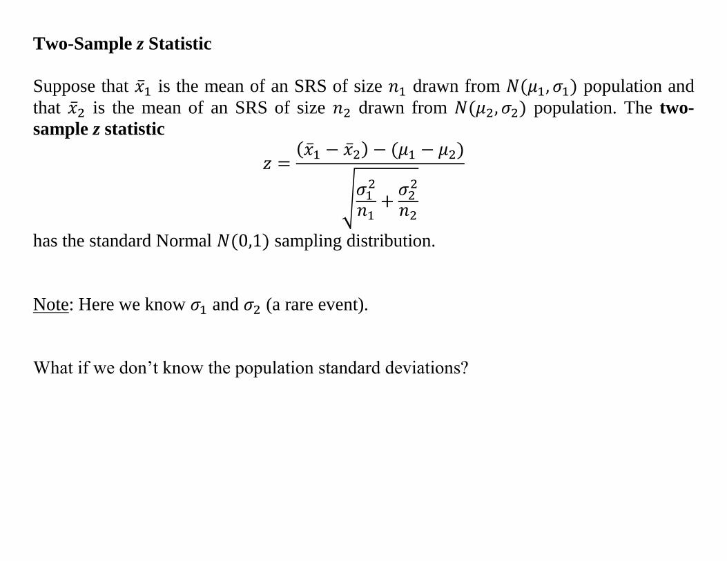
Two-Sample z Statistic

Suppose that is the mean of an SRS of size drawn from population and

that is the mean of an SRS of size drawn from population. The two-

sample z statistic

√

has the standard Normal sampling distribution.

Note: Here we know and (a rare event).

What if we don’t know the population standard deviations?

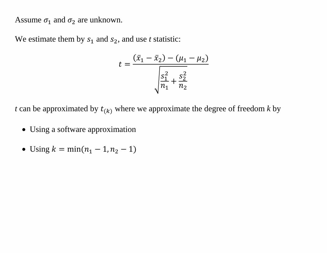
Assume and are unknown.

We estimate them by and , and use t statistic:

√

t can be approximated by where we approximate the degree of freedom k by

Using a software approximation

Using

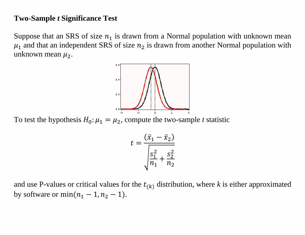
Two-Sample t Significance Test

Suppose that an SRS of size is drawn from a Normal population with unknown mean

and that an independent SRS of size is drawn from another Normal population with

unknown mean .

To test the hypothesis , compute the two-sample t statistic

√

and use P-values or critical values for the distribution, where k is either approximated

by software or .

Example: An educator believes that new directed reading activities in the classroom will

help elementary school pupils improve some aspects of their reading ability.

She arranges for a third-grade class of 21 students to take part in these activities for an

eight-week period. A control classroom of 23 third-graders follows the same curriculum

without the activities. At the end of the eight weeks, all students are given a Degree of

Reading Power (DRP) test, which measures the aspects of reading ability that the

treatment is designed to improve. The data appear in the table below:

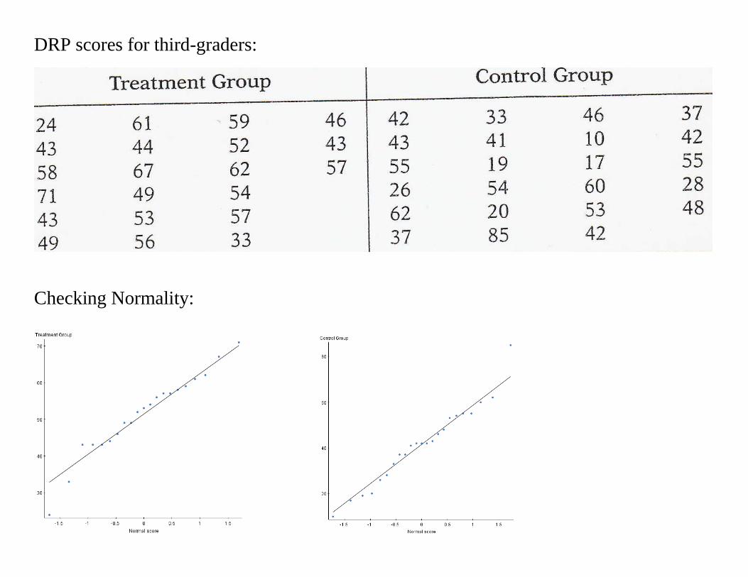
DRP scores for third-graders:

Checking Normality:

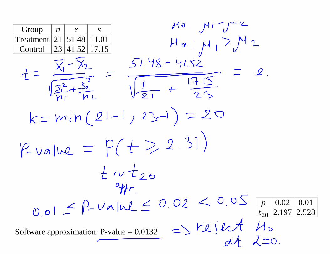
Group n s

Treatment 21 51.48 11.01

Control 23 41.52 17.15

p 0.02 0.01

2.197 2.528

Software approximation: P-value = 0.0132

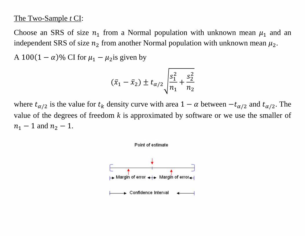
The Two-Sample t CI:

Choose an SRS of size from a Normal population with unknown mean and an

independent SRS of size from another Normal population with unknown mean .

A CI for is given by

√

where is the value for density curve with area between and . The

value of the degrees of freedom k is approximated by software or we use the smaller of

and .

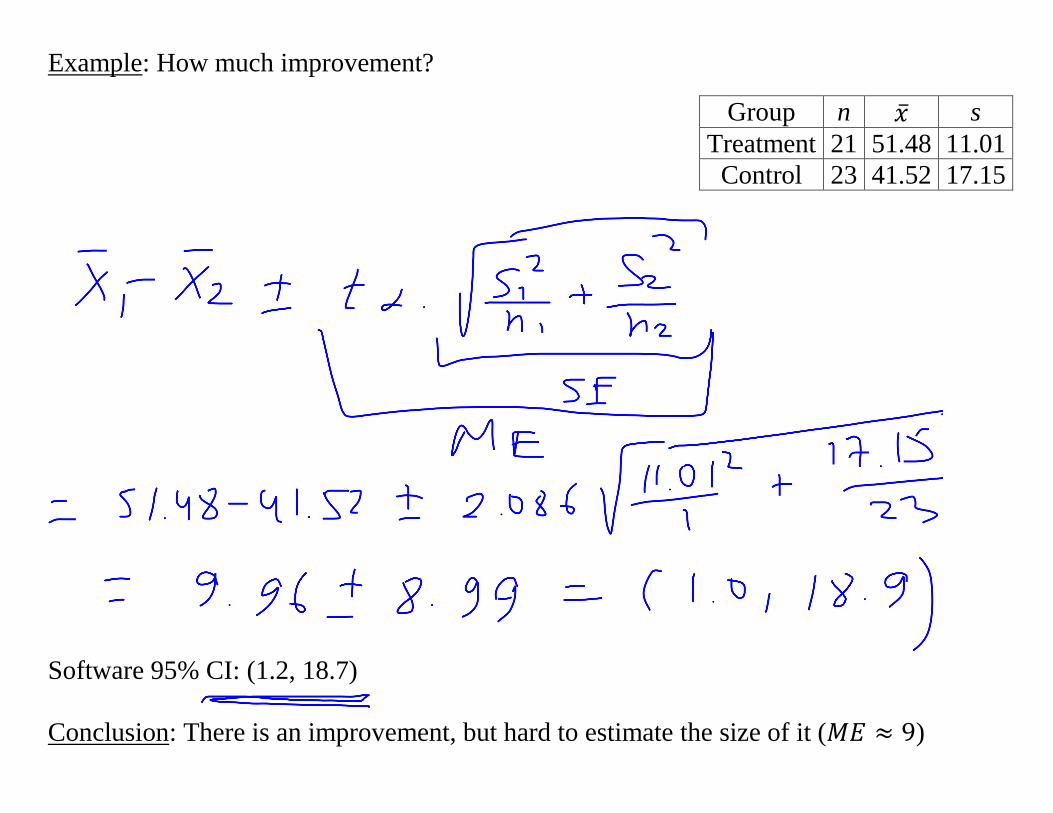
Example: How much improvement?

Group n s

Treatment 21 51.48 11.01

Control 23 41.52 17.15

Software 95% CI: (1.2, 18.7)

Conclusion: There is an improvement, but hard to estimate the size of it ( )

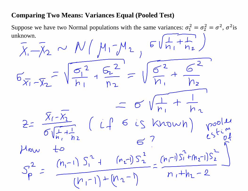
Comparing Two Means: Variances Equal (Pooled Test)

Suppose we have two Normal populations with the same variances:

, is

unknown.

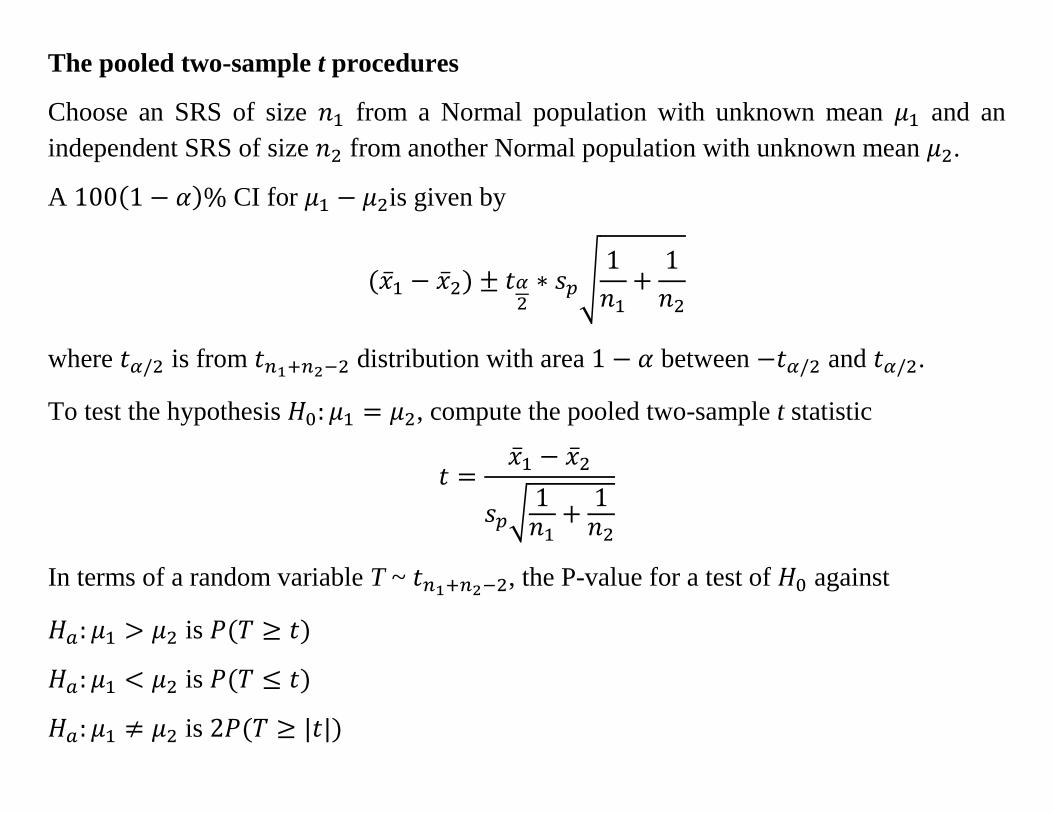
The pooled two-sample t procedures

Choose an SRS of size from a Normal population with unknown mean and an

independent SRS of size from another Normal population with unknown mean .

A CI for is given by

√

where is from distribution with area between and .

To test the hypothesis , compute the pooled two-sample t statistic

√

In terms of a random variable T ~ , the P-value for a test of against

is

is

is

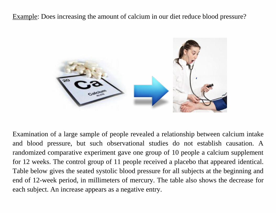
Example: Does increasing the amount of calcium in our diet reduce blood pressure?

Examination of a large sample of people revealed a relationship between calcium intake

and blood pressure, but such observational studies do not establish causation. A

randomized comparative experiment gave one group of 10 people a calcium supplement

for 12 weeks. The control group of 11 people received a placebo that appeared identical.

Table below gives the seated systolic blood pressure for all subjects at the beginning and

end of 12-week period, in millimeters of mercury. The table also shows the decrease for

each subject. An increase appears as a negative entry.

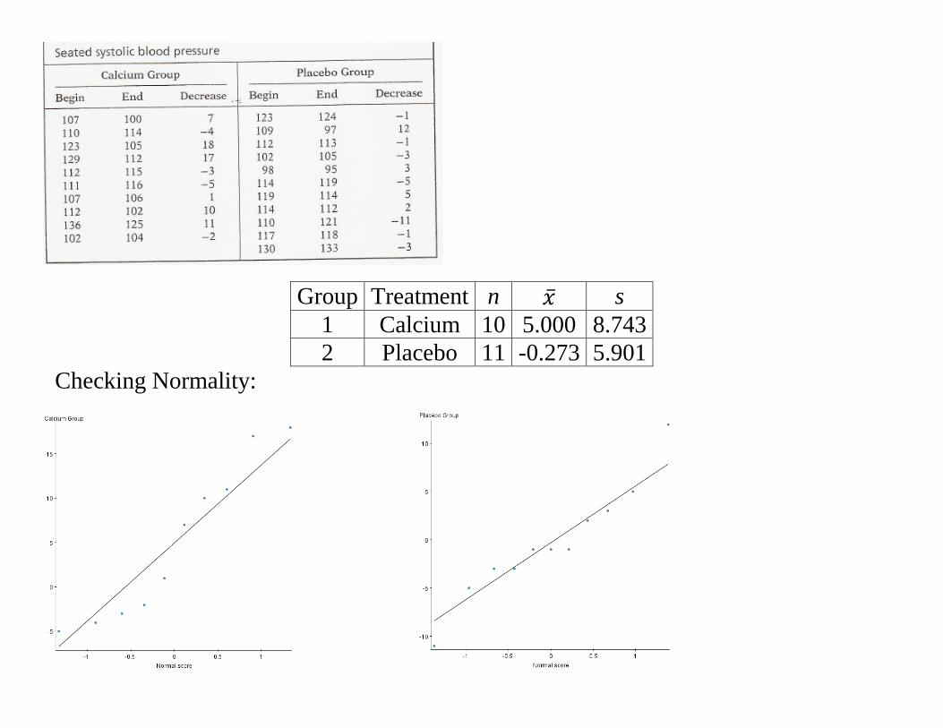
Group Treatment n s

1 Calcium 10 5.000 8.743

2 Placebo 11 -0.273 5.901

Checking Normality:

Does increased calcium reduce blood pressure?

Group Treatment n s

1 Calcium 10 5.000 8.743

2 Placebo 11 -0.273 5.901

p 0.10 0.05

1.328 1.729

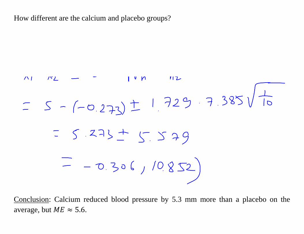
How different are the calcium and placebo groups?

Conclusion: Calcium reduced blood pressure by 5.3 mm more than a placebo on the

average, but .

Inference for Non-Normal Population

Question: How to do inference about the mean of a clearly non-Normal distribution based

on a small sample?

Three general strategies are available:

In some cases a distribution other than a Normal distribution will describe the data

well. There are many non-Normal models for data, and inference procedures for

these models are available.

Because skewness is the chief barrier to the use of t procedures on data without

outliers, you can attempt to transform skewed data so that the distribution is

symmetric and as close to Normal as possible. Confidence levels and P-values from t

procedures applied to the transformed data will be quite accurate for even moderate

sample sizes.

Use a distribution-free inference procedure. Such procedures do not assume that the

population distribution has any specific form, such as Normal. Distribution-free

procedures are often called nonparametric procedures.

Distribution-free tests have two drawbacks:

They are less powerful

We must often modify the statement of the hypotheses

The simplest distribution-free test is the sign test.

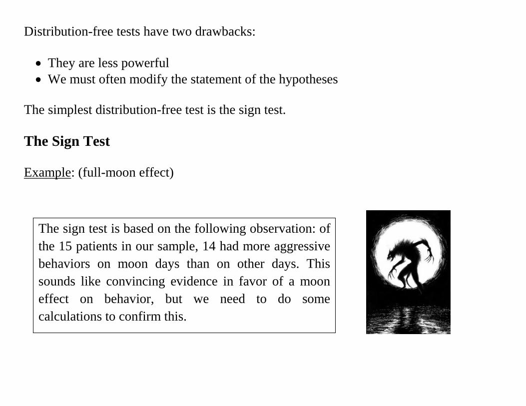
The Sign Test

Example: (full-moon effect)

The sign test is based on the following observation: of

the 15 patients in our sample, 14 had more aggressive

behaviors on moon days than on other days. This

sounds like convincing evidence in favor of a moon

effect on behavior, but we need to do some

calculations to confirm this.

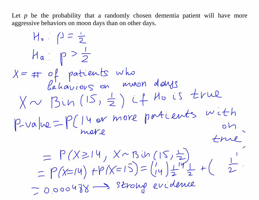
Let p be the probability that a randomly chosen dementia patient will have more

aggressive behaviors on moon days than on other days.

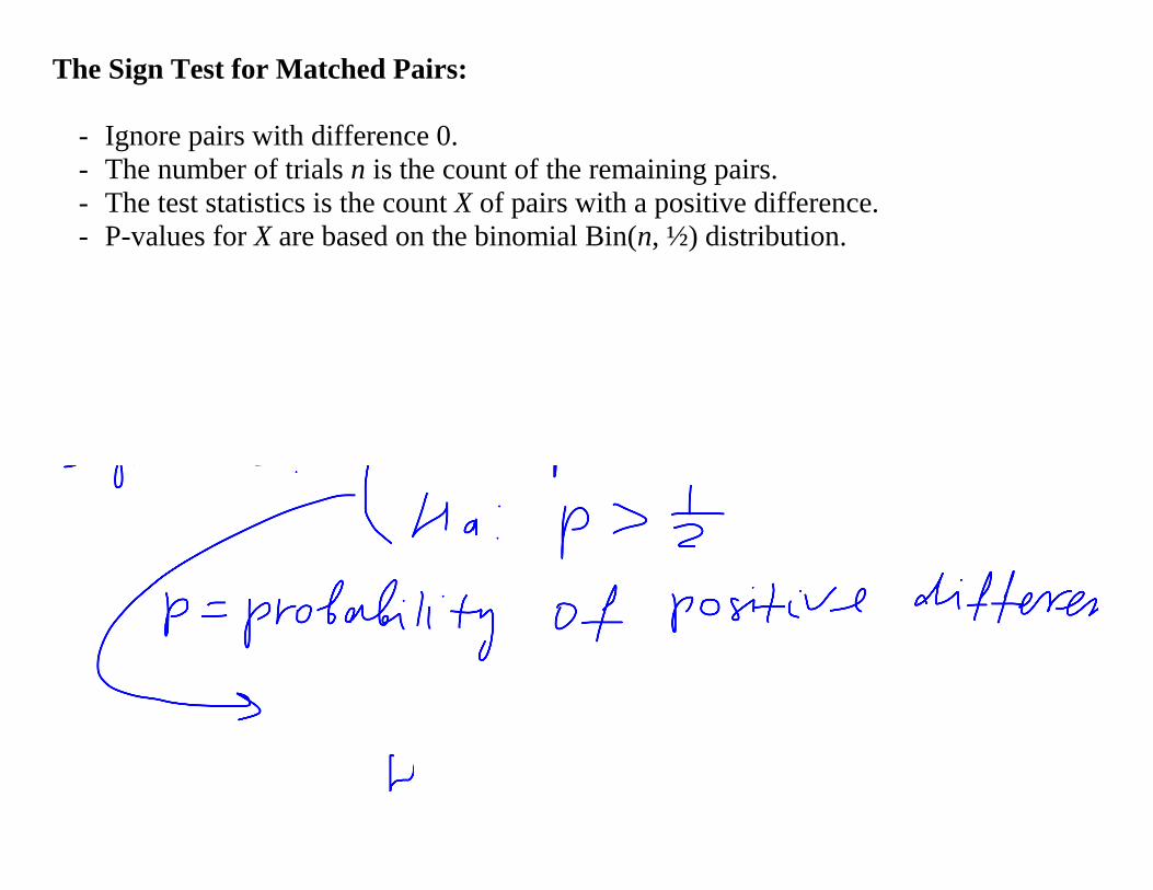
The Sign Test for Matched Pairs:

- Ignore pairs with difference 0.

- The number of trials n is the count of the remaining pairs.

- The test statistics is the count X of pairs with a positive difference.

- P-values for X are based on the binomial Bin(n, ½) distribution.