Lecture 10 The primary goal for a speech recognition ...
22
Lecture 10 Discriminative Training, ROVER, and Consensus Michael Picheny, Bhuvana Ramabhadran, Stanley F. Chen IBM T.J. Watson Research Center Yorktown Heights, New York, USA {picheny,bhuvana,stanchen}@us.ibm.com 10 December 2012 General Motivation The primary goal for a speech recognition system is to accurately recognize the words. The modeling and adaptation techniques we have studied till now implicitly address this goal. Today we will focus on techniques explicitly targeted to improving accuracy. 2 / 86 Where Are We? 1 Linear Discriminant Analysis 2 Maximum Mutual Information Estimation 3 ROVER 4 Consensus Decoding 3 / 86 Where Are We? 1 Linear Discriminant Analysis LDA - Motivation Eigenvectors and Eigenvalues PCA - Derivation LDA - Derivation Applying LDA to Speech Recognition 4 / 86
Transcript of Lecture 10 The primary goal for a speech recognition ...
Lecture 10
Discriminative Training, ROVER, and Consensus
Michael Picheny, Bhuvana Ramabhadran, Stanley F. Chen
IBM T.J. Watson Research CenterYorktown Heights, New York, USA
{picheny,bhuvana,stanchen}@us.ibm.com
10 December 2012
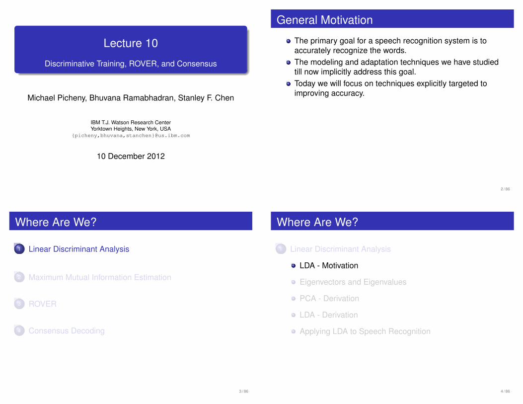
General Motivation
The primary goal for a speech recognition system is toaccurately recognize the words.The modeling and adaptation techniques we have studiedtill now implicitly address this goal.Today we will focus on techniques explicitly targeted toimproving accuracy.
2 / 86
Where Are We?
1 Linear Discriminant Analysis
2 Maximum Mutual Information Estimation
3 ROVER
4 Consensus Decoding
3 / 86
Where Are We?
1 Linear Discriminant Analysis
LDA - Motivation
Eigenvectors and Eigenvalues
PCA - Derivation
LDA - Derivation
Applying LDA to Speech Recognition
4 / 86

Linear Discriminant Analysis - Motivation
In a typical HMM using Gaussian Mixture Models we assumediagonal covariances.
This assumes that the classes to be discriminated between liealong the coordinate axes:
What if that is NOT the case?5 / 86
Principle Component Analysis-Motivation
We are in trouble.
First, we can try to rotate the coordinate axes to better lie alongthe main sources of variation.
6 / 86
Linear Discriminant Analysis - Motivation
If the main sources of class variation do NOT lie along the mainsource of variation we need to find the best directions:
7 / 86
Linear Discriminant Analysis - Computation
How do we find the best directions?
8 / 86
Where Are We?
1 Linear Discriminant Analysis
LDA - Motivation
Eigenvectors and Eigenvalues
PCA - Derivation
LDA - Derivation
Applying LDA to Speech Recognition
9 / 86
Eigenvectors and Eigenvalues
A key concept in finding good directions are the eigenvalues andeigenvectors of a matrix.
The eigenvalues and eigenvectors of a matrix are defined by thefollowing matrix equation:
Ax = λx
For a given matrix A the eigenvectors are defined as thosevectors x for which the above statement is true. Eacheigenvector has an associated eigenvalue, λ.
10 / 86
Eigenvectors and Eigenvalues - continued
To solve this equation, we can rewrite it as
(A − λI)x = 0
If xis non-zero, the only way this equation can be solved is if thedeterminant of the matrix (A − λI) is zero.
The determinant of this matrix is a polynomial (called thecharacteristic polynomial) p(λ).
The roots of this polynomial will be the eigenvalues of A.
11 / 86
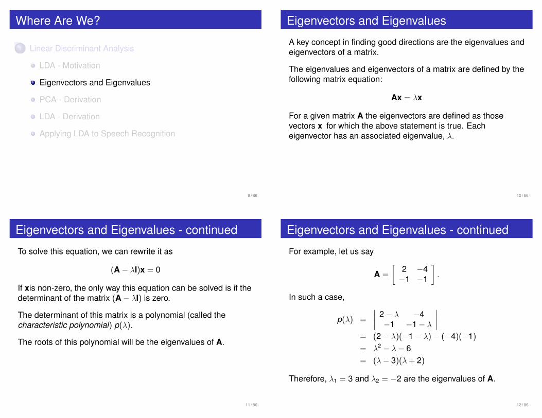
Eigenvectors and Eigenvalues - continued
For example, let us say
A =
[2 −4−1 −1
].
In such a case,
p(λ) =
∣∣∣∣ 2 − λ −4−1 −1 − λ
∣∣∣∣= (2 − λ)(−1 − λ) − (−4)(−1)
= λ2 − λ − 6= (λ − 3)(λ + 2)
Therefore, λ1 = 3 and λ2 = −2 are the eigenvalues of A.
12 / 86
Eigenvectors and Eigenvalues - continued
To find the eigenvectors, we simply plug in the eigenvalues into(A − λI)x = 0 and solve for x. For example, for λ1 = 3 we get[
2 − 3 −4−1 −1 − 3
] [x1
x2
]=
[00
]Solving this, we find that x1 = −4x2, so all the eigenvectorcorresponding to λ1 = 3 is a multiple of [−4 1]T .
Similarly, we find that the eigenvector corresponding to λ1 = −2is a multiple of [1 1]T .
13 / 86
Where Are We?
1 Linear Discriminant Analysis
LDA - Motivation
Eigenvectors and Eigenvalues
PCA - Derivation
LDA - Derivation
Applying LDA to Speech Recognition
14 / 86
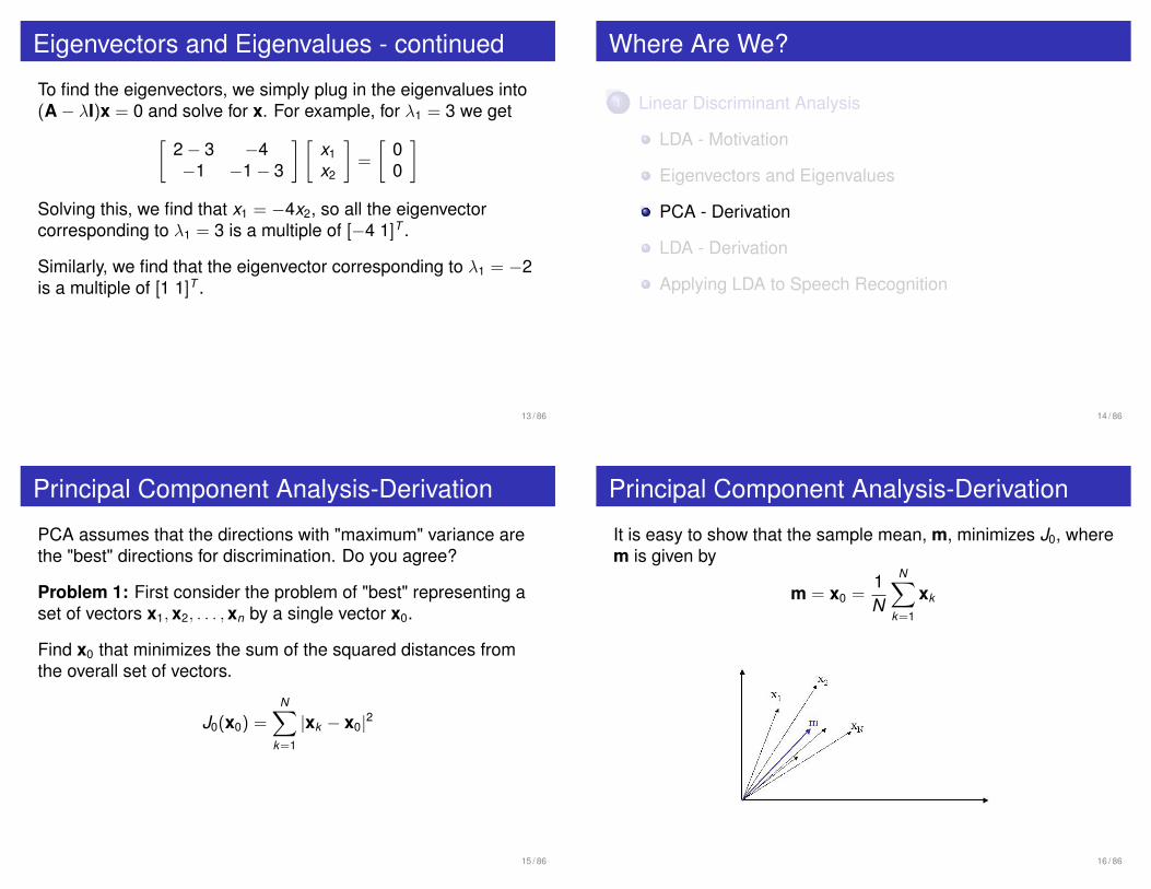
Principal Component Analysis-Derivation
PCA assumes that the directions with "maximum" variance arethe "best" directions for discrimination. Do you agree?
Problem 1: First consider the problem of "best" representing aset of vectors x1, x2, . . . , xn by a single vector x0.
Find x0 that minimizes the sum of the squared distances fromthe overall set of vectors.
J0(x0) =N∑
k=1
|xk − x0|2
15 / 86
Principal Component Analysis-Derivation
It is easy to show that the sample mean, m, minimizes J0, wherem is given by
m = x0 =1N
N∑k=1
xk
16 / 86
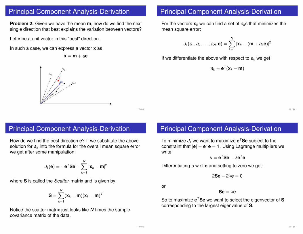
Principal Component Analysis-Derivation
Problem 2: Given we have the mean m, how do we find the nextsingle direction that best explains the variation between vectors?
Let e be a unit vector in this "best" direction.
In such a case, we can express a vector x as
x = m + ae
17 / 86
Principal Component Analysis-Derivation
For the vectors xk we can find a set of aks that minimizes themean square error:
J1(a1, a2, . . . , aN , e) =N∑
k=1
|xk − (m + ake)|2
If we differentiate the above with respect to ak we get
ak = eT (xk − m)
18 / 86
Principal Component Analysis-Derivation
How do we find the best direction e? If we substitute the abovesolution for ak into the formula for the overall mean square errorwe get after some manipulation:
J1(e) = −eT Se +N∑
k=1
|xk − m|2
where S is called the Scatter matrix and is given by:
S =N∑
k=1
(xk − m)(xk − m)T
Notice the scatter matrix just looks like N times the samplecovariance matrix of the data.
19 / 86
Principal Component Analysis-Derivation
To minimize J1 we want to maximize eT Se subject to theconstraint that |e| = eT e = 1. Using Lagrange multipliers wewrite
u = eT Se − λeT e
Differentiating u w.r.t e and setting to zero we get:
2Se − 2λe = 0
orSe = λe
So to maximize eT Se we want to select the eigenvector of Scorresponding to the largest eigenvalue of S.
20 / 86
Principal Component Analysis-Derivation
Problem 3: How do we find the best d directions?
Express x as
x = m +d∑
i=1
aiei
In this case, we can write the mean square error as
Jd =N∑
k=1
|(m +d∑
i=1
akiei) − xk |2
and it is not hard to show that Jd is minimized when the vectorse1, e2, . . . , ed correspond to the d largest eigenvectors of thescatter matrix S.
21 / 86
Where Are We?
1 Linear Discriminant Analysis
LDA - Motivation
Eigenvectors and Eigenvalues
PCA - Derivation
LDA - Derivation
Applying LDA to Speech Recognition
22 / 86
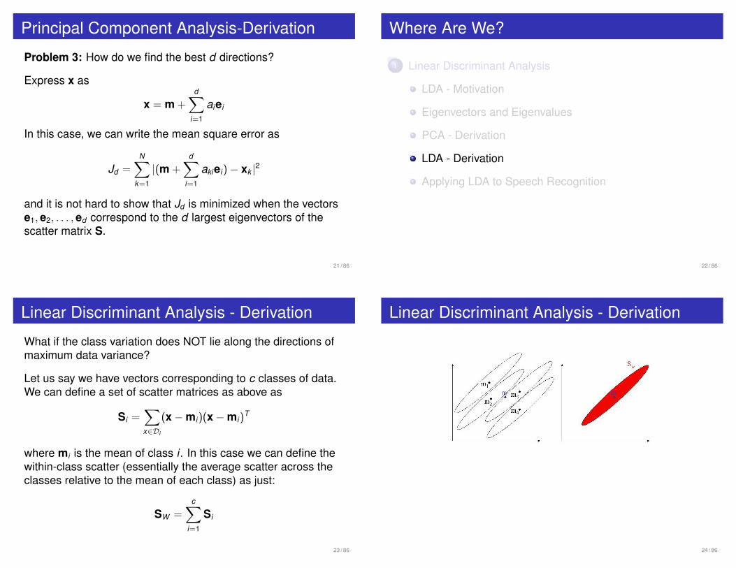
Linear Discriminant Analysis - Derivation
What if the class variation does NOT lie along the directions ofmaximum data variance?
Let us say we have vectors corresponding to c classes of data.We can define a set of scatter matrices as above as
Si =∑x∈Di
(x − mi)(x − mi)T
where mi is the mean of class i . In this case we can define thewithin-class scatter (essentially the average scatter across theclasses relative to the mean of each class) as just:
SW =c∑
i=1
Si
23 / 86
Linear Discriminant Analysis - Derivation
24 / 86
Linear Discriminant Analysis - Derivation
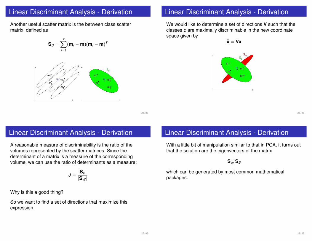
Another useful scatter matrix is the between class scattermatrix, defined as
SB =c∑
i=1
(mi − m)(mi − m)T
25 / 86
Linear Discriminant Analysis - Derivation
We would like to determine a set of directions V such that theclasses c are maximally discriminable in the new coordinatespace given by
x̃ = Vx
26 / 86
Linear Discriminant Analysis - Derivation
A reasonable measure of discriminability is the ratio of thevolumes represented by the scatter matrices. Since thedeterminant of a matrix is a measure of the correspondingvolume, we can use the ratio of determinants as a measure:
J =|SB||SW |
Why is this a good thing?
So we want to find a set of directions that maximize thisexpression.
27 / 86
Linear Discriminant Analysis - Derivation
With a little bit of manipulation similar to that in PCA, it turns outthat the solution are the eigenvectors of the matrix
S−1W SB
which can be generated by most common mathematicalpackages.
28 / 86

Where Are We?
1 Linear Discriminant Analysis
LDA - Motivation
Eigenvectors and Eigenvalues
PCA - Derivation
LDA - Derivation
Applying LDA to Speech Recognition
29 / 86
Linear Discriminant Analysis in SpeechRecognition
The most successful uses of LDA in speech recognition areachieved in an interesting fashion.
Speech recognition training data are aligned against theunderlying words using the Viterbi alignment algorithmdescribed in Lecture 4.Using this alignment, each cepstral vector is tagged with adifferent phone or sub-phone. For English this typicallyresults in a set of 156 (52x3) classes.For each time t the cepstral vector xt is spliced togetherwith N/2 vectors on the left and right to form a“supervector” of N cepstral vectors. (N is typically 5-9frames.) Call this “supervector” yt .
30 / 86
Linear Discriminant Analysis in SpeechRecognition
31 / 86
Linear Discriminant Analysis in SpeechRecognition
The LDA procedure is applied to the supervectors yt .The top M directions (usually 40-60) are chosen and thesupervectors yt are projected into this lower dimensionalspace.The recognition system is retrained on these lowerdimensional vectors.Performance improvements of 10%-15% are typical.Almost no additional computational or memory cost!
32 / 86
Where Are We?
1 Linear Discriminant Analysis
2 Maximum Mutual Information Estimation
3 ROVER
4 Consensus Decoding
33 / 86
Where Are We?
2 Maximum Mutual Information Estimation
Discussion of ML Estimation
Basic Principles of MMI Estimation
Overview of MMI Training Algorithm
Variations on MMI Training
34 / 86
Training via Maximum Mutual Information
Fundamental Equation of Speech Recognition:
p(S|O) =p(O|S)p(S)
P(O)
where S is the sentence and O are our observations. p(O|S)has a set of parameters θ that are estimated from a set oftraining data, so we write this dependence explicitly: pθ(O|S).
We estimate the parameters θ to maximize the likelihood of thetraining data. Is this the best thing to do?
35 / 86
Main Problem with Maximum LikelihoodEstimation
The true distribution of speech is (probably) not generated by anHMM, at least not of the type we are currently using.
Therefore, the optimality of the ML estimate is not guaranteedand the parameters estimated may not result in the lowest errorrates.
Rather than maximizing the likelihood of the data given themodel, we can try to maximize the a posteriori probability of themodel given the data:
θMMI = arg maxθ
pθ(S|O)
36 / 86
Where Are We?
2 Maximum Mutual Information Estimation
Discussion of ML Estimation
Basic Principles of MMI Estimation
Overview of MMI Training Algorithm
Variations on MMI Training
37 / 86
MMI Estimation
It is more convenient to look at the problem as maximizing thelogarithm of the a posteriori probability across all the sentences:
θMMI = arg maxθ
∑i
log pθ(Si |Oi)
= arg maxθ
∑i
logpθ(Oi |Si)p(Si)
pθ(Oi)
= arg maxθ
∑i
logpθ(Oi |Si)p(Si)∑j pθ(Oi |S j
i )p(S ji )
where S ji refers to the j th possible sentence hypothesis given a
set of acoustic observations Oi
38 / 86
Comparison to ML Estimation
In ordinary ML estimation, the objective is to find θ :
θML = arg maxθ
∑i
log pθ(Oi |Si)
Advantages:
Only need to make computations over correct sentence.Simple algorithm (F-B) for estimating θ
MMI much more complicated.
39 / 86
Administrivia
Make-up class: Wednesday, 4:10–6:40pm, right here.Deep Belief Networks!
Lab 4 to be handed back Wednesday.Next Monday: presentations for non-reading projects.Papers due next Monday, 11:59pm.
Submit via Courseworks DropBox.
40 / 86
Where Are We?
2 Maximum Mutual Information Estimation
Discussion of ML Estimation
Basic Principles of MMI Estimation
Overview of MMI Training Algorithm
Variations on MMI Training
41 / 86
MMI Training Algorithm
A forward-backward-like algorithm exists for MMI training [2].
Derivation complex but resulting estimation formulas aresurprisingly simple.
We will just present formulae for the means.
42 / 86
MMI Training Algorithm
The MMI objective function is∑i
logpθ(Oi |Si)p(Si)∑j pθ(Oi |S j
i )p(S ji )
We can view this as comprising two terms, the numerator, andthe denominator.
We can increase the objective function in two ways:
Increase the contribution from the numerator term.Decrease the contribution from the denominator term.
Either way this has the effect of increasing the probability of thecorrect hypothesis relative to competing hypotheses.
43 / 86
MMI Training Algorithm
Let
Θnummk =
∑i,t
Oi(t)γnummki (t)
Θdenmk =
∑i,t
Oi(t)γdenmki (t)
γnummki (t) are the observation counts for state k , mixture
component m, computed from running the forward-backwardalgorithm on the “correct” sentence Si and
γdenmki (t) are the counts computed across all the sentence
hypotheses for Si
Review: What do we mean by counts?
44 / 86
MMI Training Algorithm
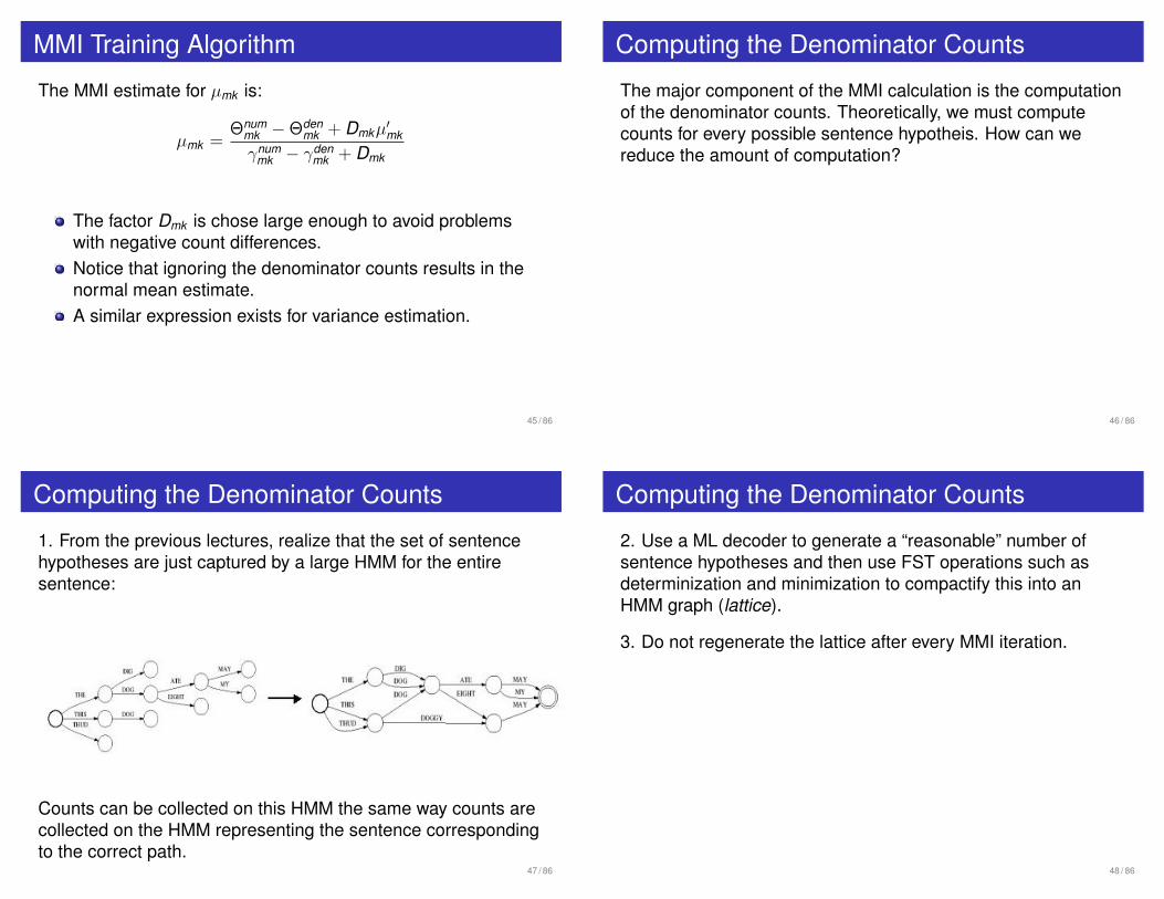
The MMI estimate for µmk is:
µmk =Θnum
mk − Θdenmk + Dmkµ
′mk
γnummk − γden
mk + Dmk
The factor Dmk is chose large enough to avoid problemswith negative count differences.Notice that ignoring the denominator counts results in thenormal mean estimate.A similar expression exists for variance estimation.
45 / 86
Computing the Denominator Counts
The major component of the MMI calculation is the computationof the denominator counts. Theoretically, we must computecounts for every possible sentence hypotheis. How can wereduce the amount of computation?
46 / 86
Computing the Denominator Counts
1. From the previous lectures, realize that the set of sentencehypotheses are just captured by a large HMM for the entiresentence:
Counts can be collected on this HMM the same way counts arecollected on the HMM representing the sentence correspondingto the correct path.
47 / 86
Computing the Denominator Counts
2. Use a ML decoder to generate a “reasonable” number ofsentence hypotheses and then use FST operations such asdeterminization and minimization to compactify this into anHMM graph (lattice).
3. Do not regenerate the lattice after every MMI iteration.
48 / 86
Other Computational Issues
Because we ignore correlation, the likelihood of the data tendsto be dominated by a very small number of lattice paths (Why?).
To increase the number of confusable paths, the likelihoods arescaled with an exponential constant:∑
i
logpθ(Oi |Si)
κp(Si)κ∑
j pθ(Oi |S ji )
κp(S ji )
κ
For similar reasons, a weaker language model (unigram) is usedto generate the denominator lattice. This also simplifiesdenominator lattice generation.
49 / 86
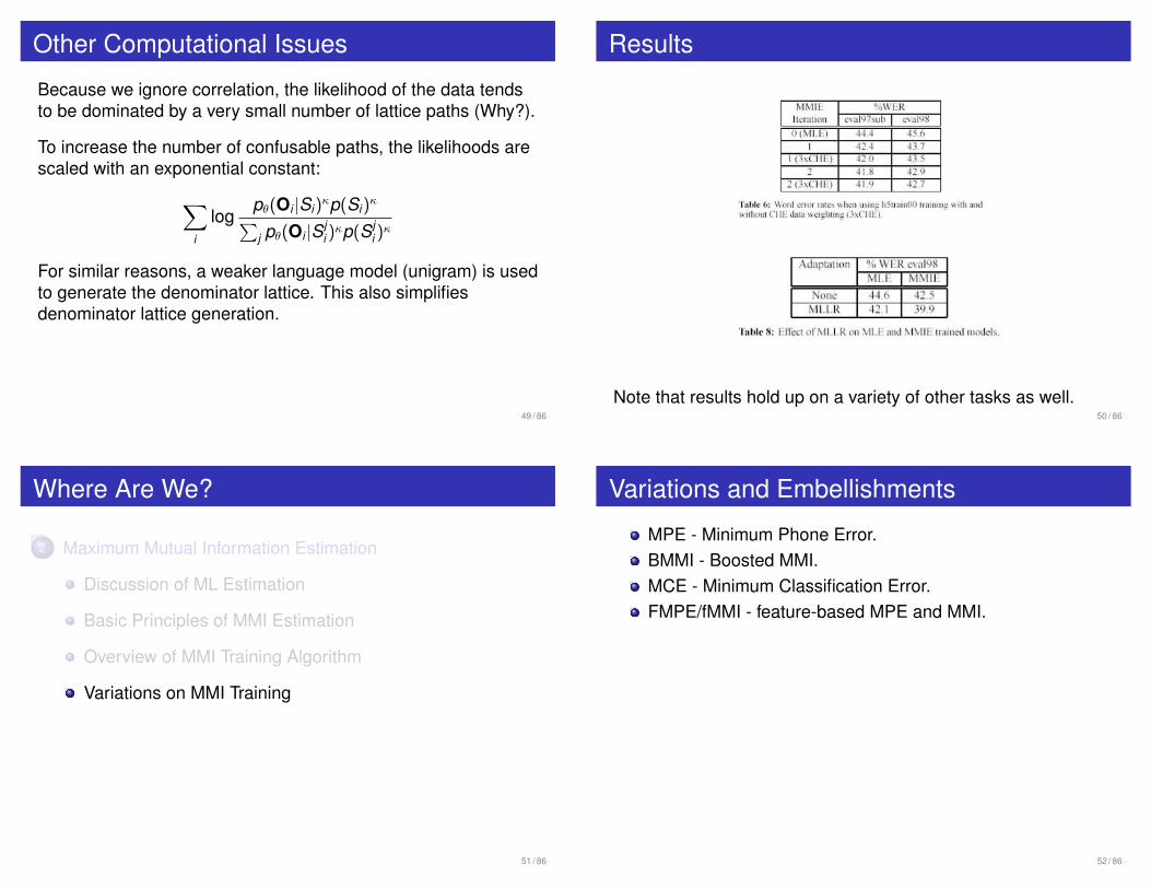
Results
Note that results hold up on a variety of other tasks as well.50 / 86
Where Are We?
2 Maximum Mutual Information Estimation
Discussion of ML Estimation
Basic Principles of MMI Estimation
Overview of MMI Training Algorithm
Variations on MMI Training
51 / 86
Variations and Embellishments
MPE - Minimum Phone Error.BMMI - Boosted MMI.MCE - Minimum Classification Error.FMPE/fMMI - feature-based MPE and MMI.
52 / 86
MPE
∑i
∑j pθ(Oi |Sj)
κp(Sj)κA(Sref , Sj)∑
j pθ(Oi |S ji )
κp(S ji )
κ
A(Sref , Sj) is a phone-frame accuracy function. A measuresthe number of correctly labeled frames in S.Povey [3] showed this could be optimized in a way similar tothat of MMI.Usually works somewhat better than MMI itself.
53 / 86
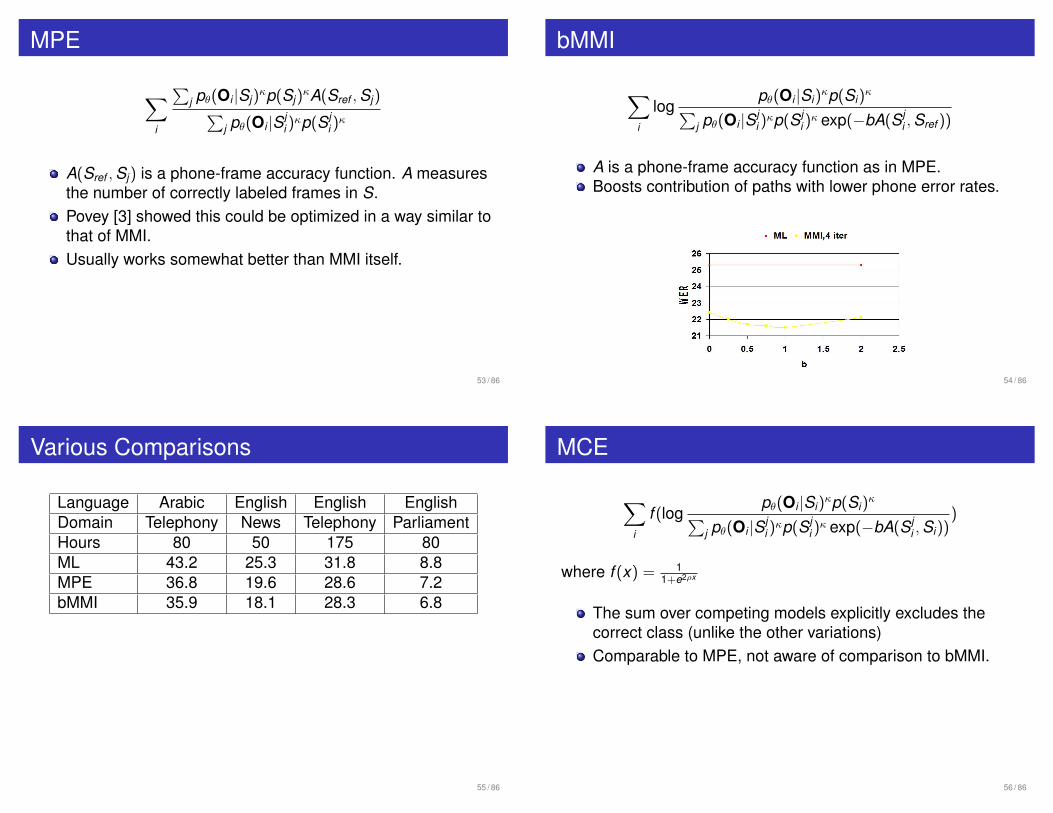
bMMI
∑i
logpθ(Oi |Si)
κp(Si)κ∑
j pθ(Oi |S ji )
κp(S ji )
κ exp(−bA(S ji , Sref ))
A is a phone-frame accuracy function as in MPE.Boosts contribution of paths with lower phone error rates.
54 / 86
Various Comparisons
Language Arabic English English EnglishDomain Telephony News Telephony ParliamentHours 80 50 175 80ML 43.2 25.3 31.8 8.8MPE 36.8 19.6 28.6 7.2bMMI 35.9 18.1 28.3 6.8
55 / 86
MCE
∑i
f (logpθ(Oi |Si)
κp(Si)κ∑
j pθ(Oi |S ji )
κp(S ji )
κ exp(−bA(S ji , Si))
)
where f (x) = 11+e2ρx
The sum over competing models explicitly excludes thecorrect class (unlike the other variations)Comparable to MPE, not aware of comparison to bMMI.
56 / 86

fMPE/fMMI
yt = Ot + Mht
ht are the set of Gaussian likelihoods for frame t . May beclustered into a smaller number of Gaussians, may also becombined across multiple frames.The training of M is exceedingly complex involving both thegradients of your favorite objective function with respect toM as well as the model parameters θ with multiple passesthrough the data.Rather amazingly gives significant gains both with andwithout MMI.
57 / 86
fMPE/fMMI Results
English BN 50 Hours, SI models
RT03 DEV04f RT04ML 17.5 28.7 25.3fBMMI 13.2 21.8 19.2fbMMI+ bMMI 12.6 21.1 18.2
Arabic BN 1400 Hours, SAT Models
DEV07 EVAL07 EVAL06ML 17.1 19.6 24.9fMPE 14.3 16.8 22.3fMPE+ MPE 12.6 14.5 20.1
58 / 86
References
P. Brown (1987) “The Acoustic Modeling Problem inAutomatic Speech Recognition”, PhD Thesis, Dept. ofComputer Science, Carnegie-Mellon University.
P.S. Gopalakrishnan, D. Kanevsky, A. Nadas, D. Nahamoo(1991) “ An Inequality for Rational Functions withApplications to Some Statistical Modeling Problems”, IEEETrans. on Acoustics, Speech and Signal Processing, 37(1)107-113, January 1991
D. Povey and P. Woodland (2002) “Minimum Phone Errorand i-smoothing for improved discriminative training”, Proc.ICASSP vol. 1 pp 105-108.
59 / 86
Where Are We?
1 Linear Discriminant Analysis
2 Maximum Mutual Information Estimation
3 ROVER
4 Consensus Decoding
60 / 86
ROVER - Recognizer Output Voting ErrorReduction[1]
Background:
Compare errors of recognizers from two different sites.Error rate performance similar - 44.9% vs 45.1%.Out of 5919 total errors, 738 are errors for only recognizer Aand 755 for only recognizer B.Suggests that some sort of voting process acrossrecognizers might reduce the overall error rate.
61 / 86
ROVER - Basic Architecture
Systems may come from multiple sites.Can be a single site with different processing schemes.
62 / 86
ROVER - Text String Alignment Process
63 / 86
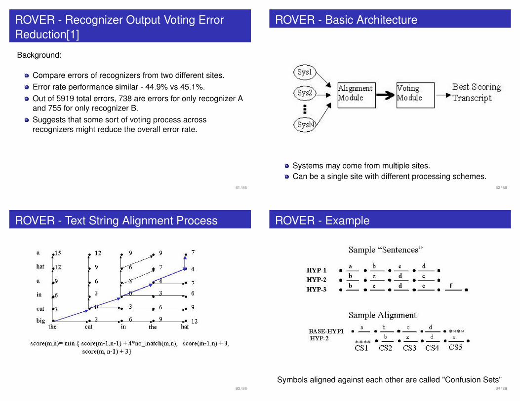
ROVER - Example
Symbols aligned against each other are called "Confusion Sets"64 / 86
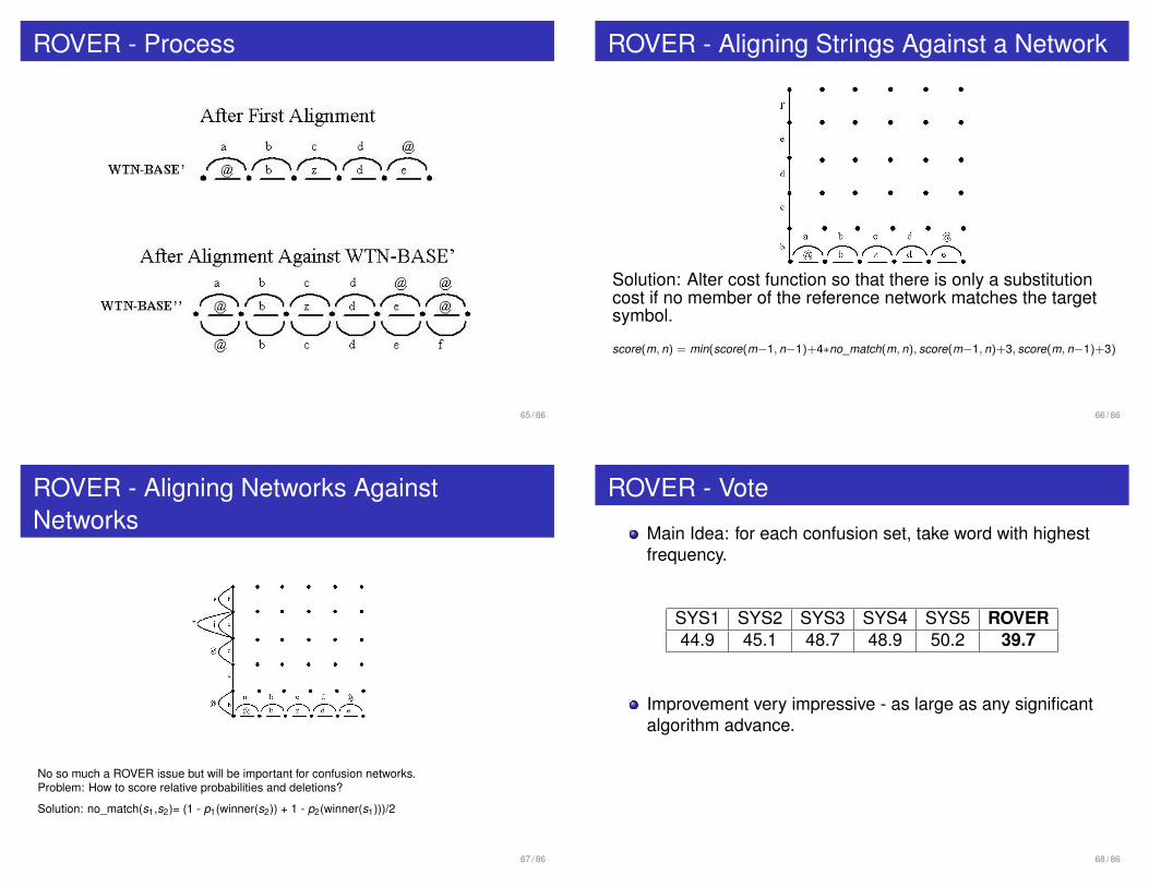
ROVER - Process
65 / 86
ROVER - Aligning Strings Against a Network
Solution: Alter cost function so that there is only a substitutioncost if no member of the reference network matches the targetsymbol.
score(m, n) = min(score(m−1, n−1)+4∗no_match(m, n), score(m−1, n)+3, score(m, n−1)+3)
66 / 86
ROVER - Aligning Networks AgainstNetworks
No so much a ROVER issue but will be important for confusion networks.Problem: How to score relative probabilities and deletions?
Solution: no_match(s1,s2)= (1 - p1(winner(s2)) + 1 - p2(winner(s1)))/2
67 / 86
ROVER - Vote
Main Idea: for each confusion set, take word with highestfrequency.
SYS1 SYS2 SYS3 SYS4 SYS5 ROVER44.9 45.1 48.7 48.9 50.2 39.7
Improvement very impressive - as large as any significantalgorithm advance.
68 / 86

ROVER - Example
Error not guaranteed to be reduced.Sensitive to initial choice of base system used for alignment- typically take the best system.
69 / 86
ROVER - As a Function of Number ofSystems [2]
Alphabetical: take systems in alphabetical order.Curves ordered by error rate.Note error actually goes up slightly with 9 systems.
70 / 86
ROVER - Types of Systems to Combine
ML and MMI.Varying amount of acoustic context in pronunciation models(Triphone, Quinphone)Different lexicons.Different signal processing schemes (MFCC, PLP).Anything else you can think of!
Rover provides an excellent way to achieve cross-sitecollaboration and synergy in a relatively painless fashion.
71 / 86
References
J. Fiscus (1997) “A Post-Processing System to YieldReduced Error Rates”, IEEE Workshop on AutomaticSpeech Recognition and Understanding, Santa Barbara, CA
H. Schwenk and J.L. Gauvain (2000) “Combining MultipleSpeech Recognizers using Voting and Language ModelInformation” ICSLP 2000, Beijing II pp. 915-918
72 / 86
Where Are We?
1 Linear Discriminant Analysis
2 Maximum Mutual Information Estimation
3 ROVER
4 Consensus Decoding
73 / 86
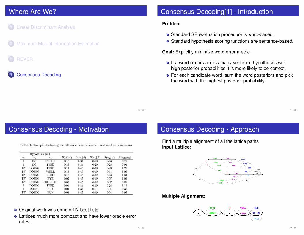
Consensus Decoding[1] - Introduction
Problem
Standard SR evaluation procedure is word-based.Standard hypothesis scoring functions are sentence-based.
Goal: Explicitly minimize word error metric
If a word occurs across many sentence hypotheses withhigh posterior probabilities it is more likely to be correct.For each candidate word, sum the word posteriors and pickthe word with the highest posterior probability.
74 / 86
Consensus Decoding - Motivation
Original work was done off N-best lists.Lattices much more compact and have lower oracle errorrates.
75 / 86
Consensus Decoding - Approach
Find a multiple alignment of all the lattice pathsInput Lattice:
SIL
SIL
SIL
SIL
SILSIL
VEAL
VERY
HAVE
HAVE
HAVE
MOVE
MOVE
HAVE
VERY
VERY
VERY
VERY
VERY
VEAL
II
I
FINE
OFTEN
OFTEN
FINE
IT
ITFAST
Multiple Alignment:
I
-VEAL
VERY
FINE
OFTEN
FAST
HAVE
-IT
MOVE
76 / 86
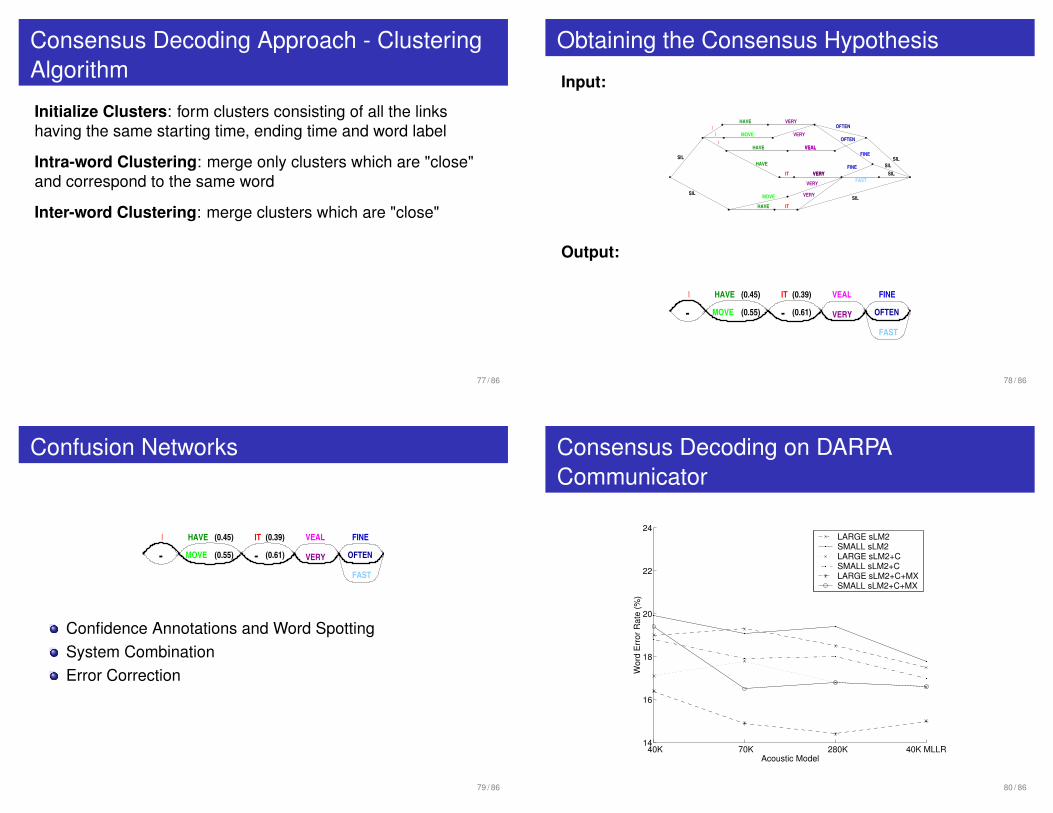
Consensus Decoding Approach - ClusteringAlgorithm
Initialize Clusters: form clusters consisting of all the linkshaving the same starting time, ending time and word label
Intra-word Clustering: merge only clusters which are "close"and correspond to the same word
Inter-word Clustering: merge clusters which are "close"
77 / 86
Obtaining the Consensus Hypothesis
Input:
SIL
SIL
SIL
SIL
SILSIL
VEAL
VERY
HAVE
HAVE
HAVE
MOVE
MOVE
HAVE
VERY
VERY
VERY
VERY
VERY
VEAL
II
I
FINE
OFTEN
OFTEN
FINE
IT
ITFAST
Output:
(0.45)
(0.55)MOVE
HAVEI
-VEAL
VERY
FINE
OFTEN
FAST
(0.39)IT
(0.61)-
78 / 86
Confusion Networks
(0.45)
(0.55)MOVE
HAVEI
-VEAL
VERY
FINE
OFTEN
FAST
(0.39)IT
(0.61)-
Confidence Annotations and Word SpottingSystem CombinationError Correction
79 / 86
Consensus Decoding on DARPACommunicator
40K 70K 280K 40K MLLR14
16
18
20
22
24
Acoustic Model
Wor
d E
rror
Rat
e (%
)
LARGE sLM2SMALL sLM2LARGE sLM2+CSMALL sLM2+CLARGE sLM2+C+MXSMALL sLM2+C+MX
80 / 86
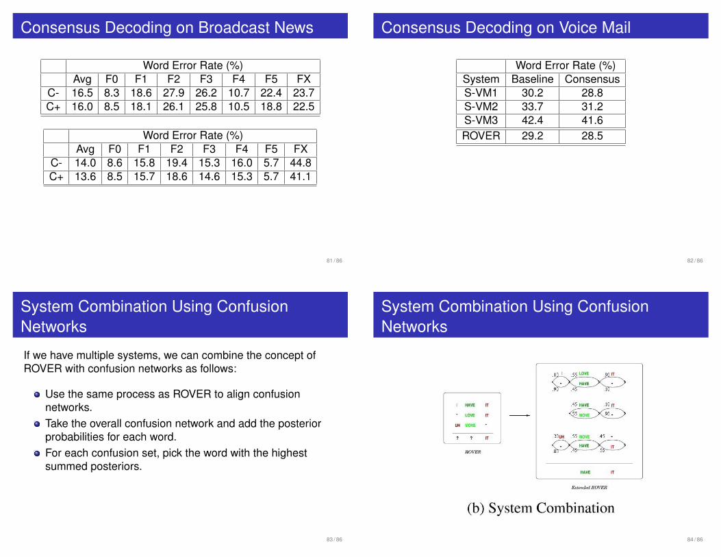
Consensus Decoding on Broadcast News
Word Error Rate (%)Avg F0 F1 F2 F3 F4 F5 FX
C- 16.5 8.3 18.6 27.9 26.2 10.7 22.4 23.7C+ 16.0 8.5 18.1 26.1 25.8 10.5 18.8 22.5
Word Error Rate (%)Avg F0 F1 F2 F3 F4 F5 FX
C- 14.0 8.6 15.8 19.4 15.3 16.0 5.7 44.8C+ 13.6 8.5 15.7 18.6 14.6 15.3 5.7 41.1
81 / 86
Consensus Decoding on Voice Mail
Word Error Rate (%)System Baseline ConsensusS-VM1 30.2 28.8S-VM2 33.7 31.2S-VM3 42.4 41.6ROVER 29.2 28.5
82 / 86
System Combination Using ConfusionNetworks
If we have multiple systems, we can combine the concept ofROVER with confusion networks as follows:
Use the same process as ROVER to align confusionnetworks.Take the overall confusion network and add the posteriorprobabilities for each word.For each confusion set, pick the word with the highestsummed posteriors.
83 / 86
System Combination Using ConfusionNetworks
84 / 86
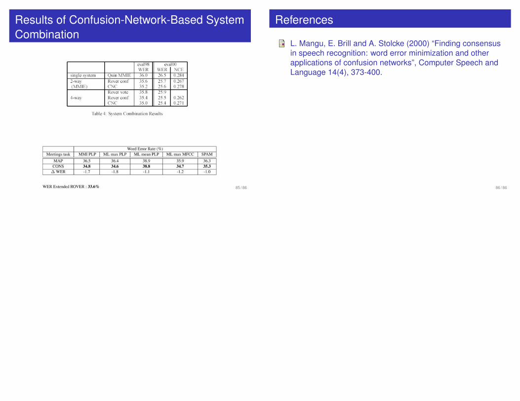
Results of Confusion-Network-Based SystemCombination
85 / 86
References
L. Mangu, E. Brill and A. Stolcke (2000) “Finding consensusin speech recognition: word error minimization and otherapplications of confusion networks”, Computer Speech andLanguage 14(4), 373-400.
86 / 86