Lecture 10 Dynamic Programming - Bilkent...
81
CS473 – Lecture 10 Cevdet Aykanat - Bilkent University Computer Engineering Department 1 CS473-Algorithms I Lecture 10 Dynamic Programming
Transcript of Lecture 10 Dynamic Programming - Bilkent...
CS473 – Lecture 10 Cevdet Aykanat - Bilkent University
Computer Engineering Department
1
CS473-Algorithms I
Lecture 10
Dynamic Programming

CS473 – Lecture 10 Cevdet Aykanat - Bilkent University
Computer Engineering Department
2
Introduction
• An algorithm design paradigm like divide-and-conquer
• “Programming”: A tabular method (not writing computer code)
• Divide-and-Conquer (DAC): subproblems are independent
• Dynamic Programming (DP): subproblems are not independent
• Overlapping subproblems: subproblems share sub-subproblems
– In solving problems with overlapping subproblems
• A DAC algorithm does redundant work
– Repeatedly solves common subproblems
• A DP algorithm solves each problem just once
– Saves its result in a table

CS473 – Lecture 10 Cevdet Aykanat - Bilkent University
Computer Engineering Department
3
Optimization Problems
• DP typically applied to optimization problems
• In an optimization problem
– There are many possible solutions (feasible solutions)
– Each solution has a value
– Want to find an optimal solution to the problem
• A solution with the optimal value (min or max value)
– Wrong to say “the” optimal solution to the problem
• There may be several solutions with the same optimal value
CS473 – Lecture 10 Cevdet Aykanat - Bilkent University
Computer Engineering Department
4
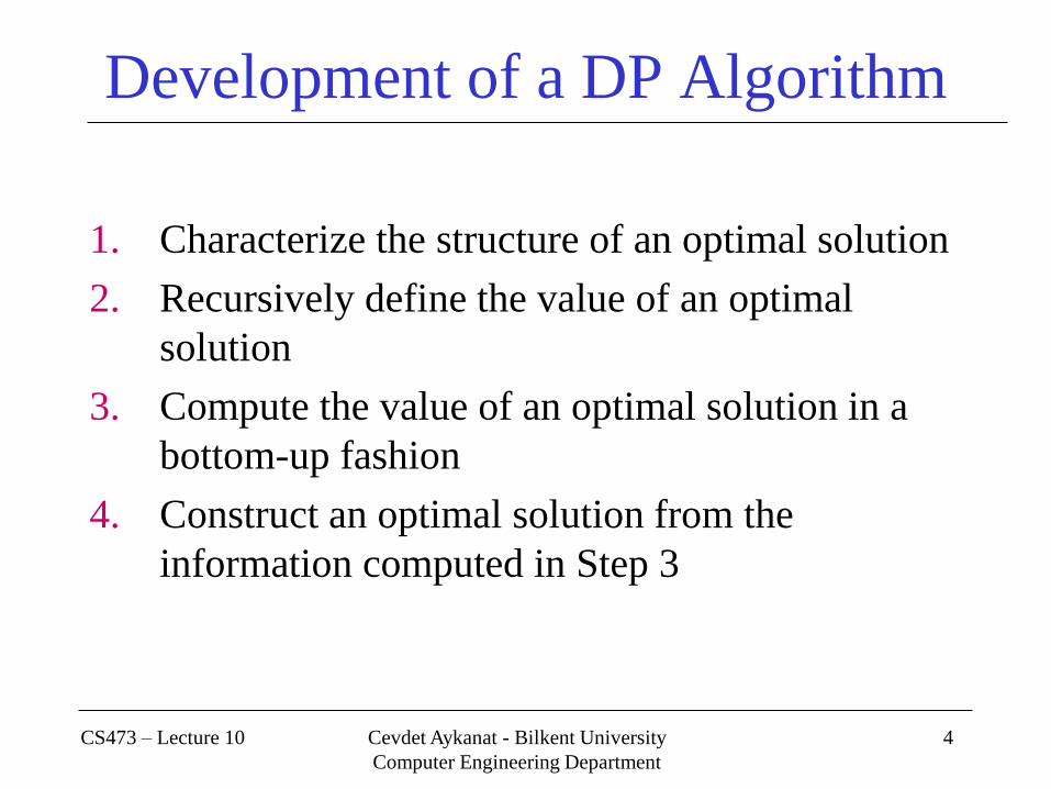
Development of a DP Algorithm
1. Characterize the structure of an optimal solution
2. Recursively define the value of an optimal
solution
3. Compute the value of an optimal solution in a
bottom-up fashion
4. Construct an optimal solution from the
information computed in Step 3
CS473 – Lecture 10 Cevdet Aykanat - Bilkent University
Computer Engineering Department
5
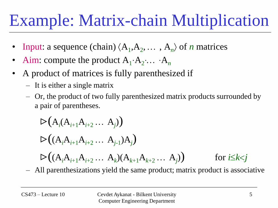
Example: Matrix-chain Multiplication
• Input: a sequence (chain) A1,A2, , An of n matrices
• Aim: compute the product A1·A2· ·An
• A product of matrices is fully parenthesized if
– It is either a single matrix
– Or, the product of two fully parenthesized matrix products surrounded by
a pair of parentheses.
(Ai(Ai+1Ai+2 Aj))
((AiAi+1Ai+2 Aj-1)Aj)
((AiAi+1Ai+2 Ak)(Ak+1Ak+2 Aj)) for ikj
– All parenthesizations yield the same product; matrix product is associative

CS473 – Lecture 10 Cevdet Aykanat - Bilkent University
Computer Engineering Department
6
Matrix-chain Multiplication: An Example
Parenthesization
• Input: A1, A2, A3, A4 • 5 distinct ways of full parenthesization
(A1(A2(A3A4)))
(A1((A2A3)A4))
((A1A2)(A3A4))
((A1(A2A3))A4)
(((A1A2)A3)A4)
• The way we parenthesize a chain of matrices can have a dramatic effect on the cost of computing the product
CS473 – Lecture 10 Cevdet Aykanat - Bilkent University
Computer Engineering Department
7
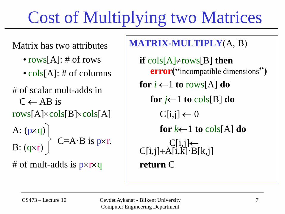
Matrix has two attributes
• rows[A]: # of rows
• cols[A]: # of columns
# of scalar mult-adds in
C AB is
rows[A]cols[B]cols[A]
A: (pq)
B: (qr)
# of mult-adds is prq
Cost of Multiplying two Matrices
MATRIX-MULTIPLY(A, B)
if cols[A]rows[B] then error(“incompatible dimensions”)
for i 1 to rows[A] do
for j1 to cols[B] do
C[i,j] 0
for k1 to cols[A] do
C[i,j] C[i,j]A[i,k]·B[k,j]
return C
C=A·B is pr.

CS473 – Lecture 10 Cevdet Aykanat - Bilkent University
Computer Engineering Department
8
Matrix-chain Multiplication Problem Input: a chain A1,A2, , An of n matrices, Ai is a pi1pi matrix
Aim: fully parenthesize the product A1 ·A2· ·An such that the number of scalar mult-adds are minimized.
• Ex.: A1, A2, A3 where A1: 10100; A2: 1005; A3: 550
((A1 A2) A3): 10 100 5 10 5 50 =7500
(A1 (A2A3)): 100550 1010050 =75000
First parenthesization yields 10 times faster computation.
105 550 A1 A2 (A1 A2)A3
10100 10050 A2 A3 A1 (A2A3)
CS473 – Lecture 10 Cevdet Aykanat - Bilkent University
Computer Engineering Department
9
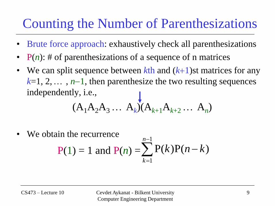
Counting the Number of Parenthesizations
• Brute force approach: exhaustively check all parenthesizations
• P(n): # of parenthesizations of a sequence of n matrices
• We can split sequence between kth and (k1)st matrices for any
k=1, 2, , n1, then parenthesize the two resulting sequences
independently, i.e.,
(A1A2A3 Ak)(Ak+1Ak+2 An)
• We obtain the recurrence
P(1) = 1 and P(n) =
1
1
)(P)(Pn
k
knk

CS473 – Lecture 10 Cevdet Aykanat - Bilkent University
Computer Engineering Department
10
Number of Parenthesizations:
• The recurrence generates the sequence of Catalan Numbers
• Solution is P(n) = C(n1) where
C(n) = = (4n/n3/2)
• The number of solutions is exponential in n
• Therefore, brute force approach is a poor strategy
1
1
)()(n
k
knPkP
1
n1
2n n
CS473 – Lecture 10 Cevdet Aykanat - Bilkent University
Computer Engineering Department
11
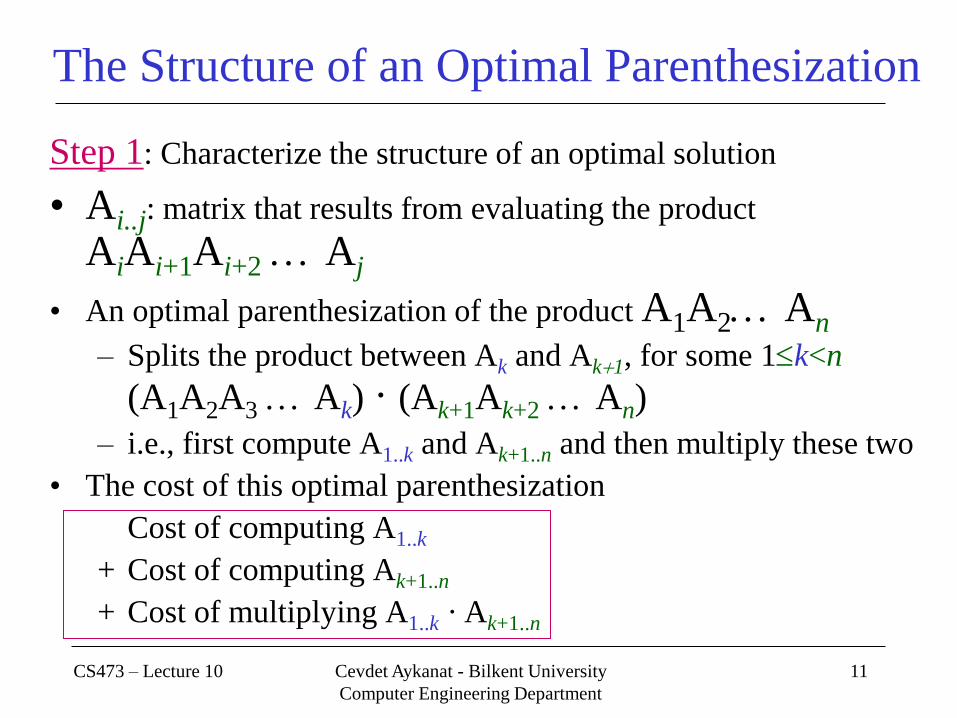
The Structure of an Optimal Parenthesization
Step 1: Characterize the structure of an optimal solution
• Ai..j: matrix that results from evaluating the product
AiAi+1Ai+2 Aj
• An optimal parenthesization of the product A1A2 An
– Splits the product between Ak and Ak1, for some 1k<n
(A1A2A3 Ak) · (Ak+1Ak+2 An)
– i.e., first compute A1..k and Ak+1..n and then multiply these two
• The cost of this optimal parenthesization
Cost of computing A1..k
+ Cost of computing Ak+1..n
+ Cost of multiplying A1..k · Ak+1..n

CS473 – Lecture 10 Cevdet Aykanat - Bilkent University
Computer Engineering Department
12
Step 1: Characterize the Structure of an Optimal Solution
• Key observation: given optimal parenthesization
(A1A2A3 Ak) · (Ak+1Ak+2 An)
– Parenthesization of the subchain A1A2A3 Ak
– Parenthesization of the subchain Ak+1Ak+2 An
should both be optimal
– Thus, optimal solution to an instance of the problem contains
optimal solutions to subproblem instances
– i.e., optimal substructure within an optimal solution exists.
CS473 – Lecture 10 Cevdet Aykanat - Bilkent University
Computer Engineering Department
13
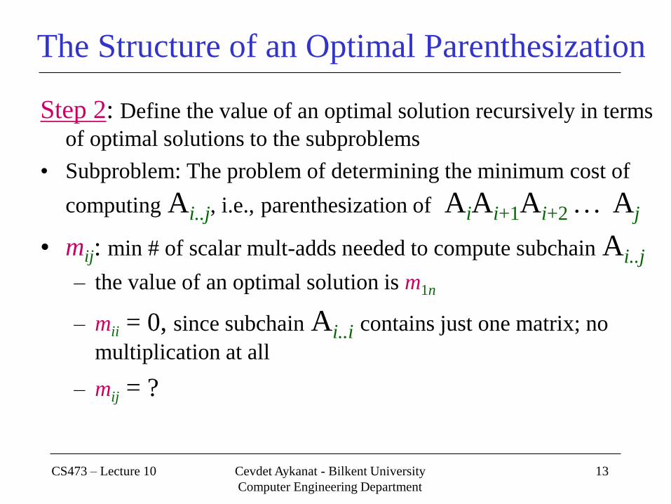
The Structure of an Optimal Parenthesization
Step 2: Define the value of an optimal solution recursively in terms
of optimal solutions to the subproblems
• Subproblem: The problem of determining the minimum cost of
computing Ai..j, i.e., parenthesization of AiAi+1Ai+2 Aj
• mij: min # of scalar mult-adds needed to compute subchain Ai..j – the value of an optimal solution is m1n
– mii = 0, since subchain Ai..i contains just one matrix; no
multiplication at all
– mij = ?
CS473 – Lecture 10 Cevdet Aykanat - Bilkent University
Computer Engineering Department
14
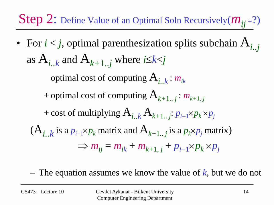
Step 2: Define Value of an Optimal Soln Recursively(mij =?)
• For i < j, optimal parenthesization splits subchain Ai..j
as Ai..k and Ak+1..j where ik<j
optimal cost of computing Ai..k : mik
+ optimal cost of computing Ak+1.. j : mk+1, j
+ cost of multiplying Ai..k Ak+1.. j: pi1pk pj
(Ai..k is a pi1pk matrix and Ak+1.. j is a pkpj matrix)
mij = mik + mk+1, j + pi1pk pj
– The equation assumes we know the value of k, but we do not

CS473 – Lecture 10 Cevdet Aykanat - Bilkent University
Computer Engineering Department
15
Step 2: Recursive Equation for mij
• mij = mik + mk+1, j + pi1pk pj
– We do not know k, but there are ji possible values
for k; k =i, i +1, i+2, …, j 1
– Since optimal parenthesization must be one of these
k values we need to check them all to find the best
0 if i=j
mij =
MIN{mik + mk+1, j +pi1pk pj} if i < j
ik<j

CS473 – Lecture 10 Cevdet Aykanat - Bilkent University
Computer Engineering Department
16
Step 2: mij = MIN{mik + mk+1, j +pi1pk pj}
• The mij values give the costs of optimal solutions
to subproblems
• In order to keep track of how to construct an
optimal solution
– Define Sij to be the value of k which yields the
optimal split of the subchain Ai..j
That is, Sij =k such that
mij = mik + mk+1, j +pi1pk pj holds

CS473 – Lecture 10 Cevdet Aykanat - Bilkent University
Computer Engineering Department
17
Computing the Optimal Cost (Matrix-Chain Multiplication)
An important observation:
• We have relatively few subproblems
one problem for each choice of i and j satisfying 1 i j n
total n (n1) … 2 1 n(n1) (n2) subproblems
• We can write a recursive algorithm based on recurrence.
• However, a recursive algorithm may encounter each subproblem
many times in different branches of the recursion tree
• This property, overlapping subproblems, is the second important
feature for applicability of dynamic programming
2
1

CS473 – Lecture 10 Cevdet Aykanat - Bilkent University
Computer Engineering Department
18
Computing the Optimal Cost (Matrix-Chain Multiplication)
Compute the value of an optimal solution in a bottom-up fashion
matrix Ai has dimensions pi1 pi for i 1, 2, …, n
the input is a sequence p0, p1, …, pn where length[p] n + 1
Procedure uses the following auxiliary tables:
m[1…n, 1…n]: for storing the m[i, j] costs
s[1…n, 1…n]: records which index of k achieved the optimal
cost in computing m[i, j]
CS473 – Lecture 10 Cevdet Aykanat - Bilkent University
Computer Engineering Department
19
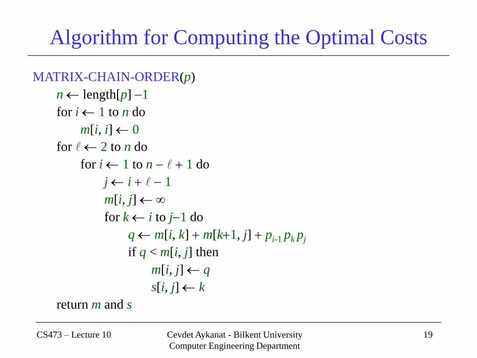
Algorithm for Computing the Optimal Costs
MATRIX-CHAIN-ORDER(p)
n length[p] 1
for i 1 to n do
m[i, i] 0
for 2 to n do
for i 1 to n 1 do
j i 1
m[i, j]
for k i to j1 do
q m[i, k] m[k1, j] pi-1 pk pj
if q < m[i, j] then
m[i, j] q
s[i, j] k
return m and s
CS473 – Lecture 10 Cevdet Aykanat - Bilkent University
Computer Engineering Department
20
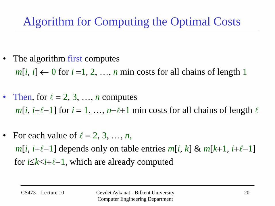
Algorithm for Computing the Optimal Costs
• The algorithm first computes
m[i, i] 0 for i 1, 2, …, n min costs for all chains of length 1
• Then, for 2, 3, …, n computes
m[i, i1] for i 1, …, n1 min costs for all chains of length
• For each value of 2, 3, …, n,
m[i, i1] depends only on table entries m[i, k] & m[k1, i1]
for ik<i1, which are already computed

CS473 – Lecture 10 Cevdet Aykanat - Bilkent University
Computer Engineering Department
21
Algorithm for Computing the Optimal Costs 2 for i 1 to n 1
m[i, i1] compute m[i, i1] for k i to i do {m[1, 2], m[2, 3], …, m[n1, n]} . . (n1) values
3 for i 1 to n 2
m[i, i2] compute m[i, i2] for k i to i1 do {m[1, 3], m[2, 4], …, m[n2, n]} . . (n2) values
4 for i 1 to n 3
m[i, i3] compute m[i, i3] for k i to i2 do {m[1, 4], m[2, 5], …, m[n3, n]} . . (n3) values

CS473 – Lecture 10 Cevdet Aykanat - Bilkent University
Computer Engineering Department
22
Table access pattern in computing m[i, j]s for ji1 Table Entries currently computed
n
1
Table entries currently computed j
1 2 3 4 . . . . i . 1 . . . . . . . . j . . . . . n
i
n1
Table entries already computed
Table entries referenced
k
k
for k i to j1 do
q m[i, k] m[k1, j] pi-1 pk
pj

CS473 – Lecture 10 Cevdet Aykanat - Bilkent University
Computer Engineering Department
23
Table access pattern in computing m[i, j]s for ji1 Table Entries currently computed
n
1
Table entries currently computed j
1 2 3 4 . . . . i . 1 . . . . . . . . j . . . . . n
i
n1
Table entries already computed
Table entries referenced
k
k
for k i to j1 do
q m[i, k] m[k1, j] pi-1 pk
pj
((Ai) (Ai+1Ai+2 Aj))

CS473 – Lecture 10 Cevdet Aykanat - Bilkent University
Computer Engineering Department
24
Table access pattern in computing m[i, j]s for ji1 Table Entries currently computed
n
1
Table entries currently computed j
1 2 3 4 . . . . i . 1 . . . . . . . . j . . . . . n
i
n1
Table entries already computed
Table entries referenced
k
k
for k i to j1 do
q m[i, k] m[k1, j] pi-1 pk
pj
((AiAi+1) (Ai+2 Aj))

CS473 – Lecture 10 Cevdet Aykanat - Bilkent University
Computer Engineering Department
25
Table access pattern in computing m[i, j]s for ji1 Table Entries currently computed
n
1
Table entries currently computed j
1 2 3 4 . . . . i . 1 . . . . . . . . j . . . . . n
i
n1
Table entries already computed
Table entries referenced
k
k
for k i to j1 do
q m[i, k] m[k1, j] pi-1 pk
pj
((AiAi+1Ai+2 ) (Ai+3Aj))
CS473 – Lecture 10 Cevdet Aykanat - Bilkent University
Computer Engineering Department
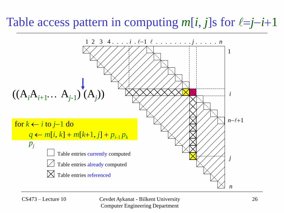
26
Table access pattern in computing m[i, j]s for ji1 Table Entries currently computed
n
1
Table entries currently computed j
1 2 3 4 . . . . i . 1 . . . . . . . . j . . . . . n
i
n1
Table entries already computed
Table entries referenced
for k i to j1 do
q m[i, k] m[k1, j] pi-1 pk
pj
((AiAi+1 Aj-1) (Aj))

CS473 – Lecture 10 Cevdet Aykanat - Bilkent University
Computer Engineering Department
27
Table reference pattern for m[i, j] (1 i j n)
m[i, j] is referenced for the computation of
m[i, r] for j < r n (n j ) times
m[r, j] for 1 r < i (i 1 ) times
Table Entries currently computed
Table entries referencing m[i, j]
The referenced table entry m[i, j]
n
1 2 3 j n
i
CS473 – Lecture 10 Cevdet Aykanat - Bilkent University
Computer Engineering Department
28
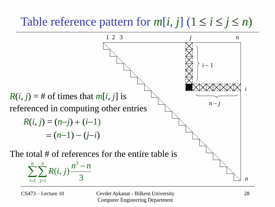
Table reference pattern for m[i, j] (1 i j n)
R(i, j) = # of times that m[i, j] is
referenced in computing other entries
R(i, j) = (nj) (i1)
(n1) (ji) The total # of references for the entire table is
Table Entries currently computed
n
1 2 3 j n
i
i 1
n j
n
i
n
ij
nnjiR
1
3
3),(
CS473 – Lecture 10 Cevdet Aykanat - Bilkent University
Computer Engineering Department
29
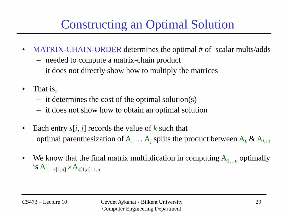
Constructing an Optimal Solution
• MATRIX-CHAIN-ORDER determines the optimal # of scalar mults/adds
needed to compute a matrix-chain product
it does not directly show how to multiply the matrices
• That is,
it determines the cost of the optimal solution(s)
it does not show how to obtain an optimal solution
• Each entry s[i, j] records the value of k such that
optimal parenthesization of Ai … Aj splits the product between Ak & Ak1
• We know that the final matrix multiplication in computing A1…n optimally is A1…s[1,n] As[1,n]1,n
CS473 – Lecture 10 Cevdet Aykanat - Bilkent University
Computer Engineering Department
30
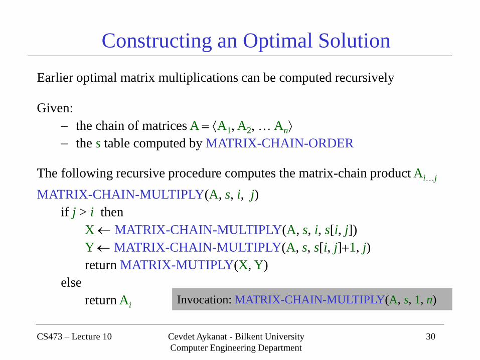
Constructing an Optimal Solution
Earlier optimal matrix multiplications can be computed recursively
Given:
the chain of matrices A A1, A2, … An
the s table computed by MATRIX-CHAIN-ORDER
The following recursive procedure computes the matrix-chain product Ai…j MATRIX-CHAIN-MULTIPLY(A, s, i, j)
if j > i then
X MATRIX-CHAIN-MULTIPLY(A, s, i, s[i, j])
Y MATRIX-CHAIN-MULTIPLY(A, s, s[i, j]1, j)
return MATRIX-MUTIPLY(X, Y)
else
return Ai
Invocation: MATRIX-CHAIN-MULTIPLY(A, s, 1, n)
CS473 – Lecture 10 Cevdet Aykanat - Bilkent University
Computer Engineering Department
31
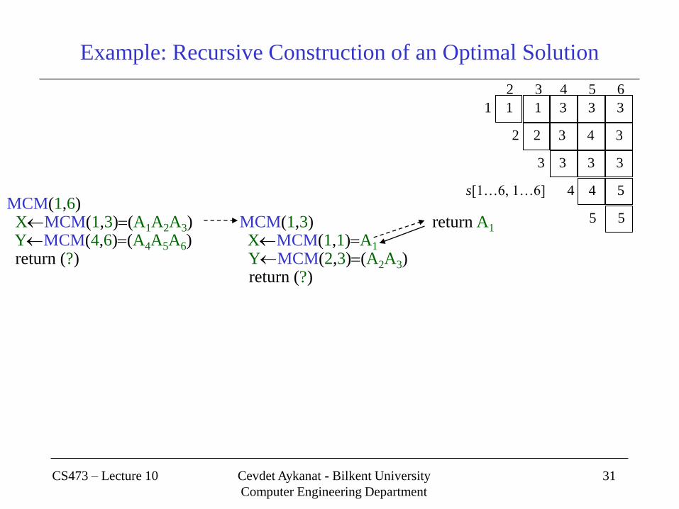
Example: Recursive Construction of an Optimal Solution MCM(1,6) XMCM(1,3)(A1A2A3) MCM(1,3) return A1 YMCM(4,6)(A4A5A6) XMCM(1,1)A1 return (?) YMCM(2,3)(A2A3) return (?)
2 3 4 5 6
1 1 1 3 3 3
2 2 3 4 3
3 3 3 3
4 4 5
5 5
s[1…6, 1…6]

CS473 – Lecture 10 Cevdet Aykanat - Bilkent University
Computer Engineering Department
32
Example: Recursive Construction of an Optimal Solution MCM(1,6) XMCM(1,3)(A1(A2A3)) MCM(1,3) return A1 YMCM(4,6)(A4A5A6) XMCM(1,1)A1 return (?) YMCM(2,3)(A2A3) MCM(2,3) return (A1(A2A3)) XMCM(2,2)A2 return A2 YMCM(3,3)A3 return A3 return (A2A3)
2 3 4 5 6
1 1 1 3 3 3
2 2 3 4 3
3 3 3 3
4 4 5
5 5
s[1…6, 1…6]

CS473 – Lecture 10 Cevdet Aykanat - Bilkent University
Computer Engineering Department
33
Example: Recursive Construction of an Optimal Solution MCM(1,6) XMCM(1,3)(A1(A2A3)) MCM(1,3) return A1 YMCM(4,6)((A4A5)A6) XMCM(1,1)A1 return (A1(A2A3))((A4A5)A6) YMCM(2,3)(A2A3) MCM(2,3) return (A1(A2A3)) XMCM(2,2)A2 return A2 YMCM(3,3)A3 return A3 return (A2A3) MCM(4,6) XMCM(4,5)(A4A5) MCM(4,5) YMCM(6,6)A6 XMCM(4,4)A4 return A4
return ((A4A5)A6 ) YMCM(5,5)A5 return A5 return (A4A5) return A6
2 3 4 5 6
1 1 1 3 3 3
2 2 3 4 3
3 3 3 3
4 4 5
5 5
s[1…6, 1…6]
CS473 – Lecture 10 Cevdet Aykanat - Bilkent University
Computer Engineering Department
34
Elements of Dynamic Programming
• When should we look for a DP solution to an
optimization problem?
• Two key ingredients for the problem
– Optimal substructure
– Overlapping subproblems
CS473 – Lecture 10 Cevdet Aykanat - Bilkent University
Computer Engineering Department
35
DP Hallmark #1
Optimal Substructure
• A problem exhibits optimal substructure
– if an optimal solution to a problem contains within
it optimal solutions to subproblems
• Example: matrix-chain-multiplication
Optimal parenthesization of A1A2 An that splits
the product between Ak and Ak1,
contains within it optimal soln’s to the problems of
parenthesizing A1A2 Ak and Ak+1Ak+2 An

CS473 – Lecture 10 Cevdet Aykanat - Bilkent University
Computer Engineering Department
36
Optimal Substructure
• The optimal substructure of a problem often suggests a
suitable space of subproblems to which DP can be
applied
• Typically, there may be several classes of subproblems
that might be considered natural
• Example: matrix-chain-multiplication
– All subchains of the input chain
We can choose an arbitrary sequence of matrices from the input chain
– However, DP based on this space solves many more
subproblems

CS473 – Lecture 10 Cevdet Aykanat - Bilkent University
Computer Engineering Department
37
Optimal Substructure
Finding a suitable space of subproblems
• Iterate on subproblem instances
• Example: matrix-chain-multiplication
– Iterate and look at the structure of optimal soln’s to
subproblems, sub-subproblems, and so forth
– Discover that all subproblems consists of subchains of
A1, A2, , An
– Thus, the set of chains of the form
Ai,Ai+1, , Aj for 1 i j n
– Makes a natural and reasonable space of subproblems

CS473 – Lecture 10 Cevdet Aykanat - Bilkent University
Computer Engineering Department
38
DP Hallmark #2
Overlapping Subproblems
• Total number of distinct subproblems should
be polynomial in the input size
• When a recursive algorithm revisits the same
problem over and over again
we say that the optimization problem has
overlapping subproblems

CS473 – Lecture 10 Cevdet Aykanat - Bilkent University
Computer Engineering Department
39
Overlapping Subproblems
• DP algorithms typically take advantage of
overlapping subproblems
– by solving each problem once
– then storing the solutions in a table
where it can be looked up when needed
– using constant time per lookup
CS473 – Lecture 10 Cevdet Aykanat - Bilkent University
Computer Engineering Department
40
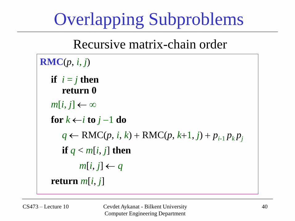
Overlapping Subproblems
Recursive matrix-chain order
RMC(p, i, j)
if i = j then return 0
m[i, j]
for k i to j 1 do
q RMC(p, i, k) RMC(p, k1, j) pi-1 pk pj
if q < m[i, j] then
m[i, j] q
return m[i, j]

CS473 – Lecture 10 Cevdet Aykanat - Bilkent University
Computer Engineering Department
41
2..2 3..4 2..3 4..4 1..1 2..2 3..3 4..4 1..1 2..3 1..2 3..3
3..3 4..4 2..2 3..3 2..2 3..3 1..1 2..2
1..1 2..4 1..2 3..4 1..3 4..4
1..4
k = 1
k = 1
k =
2k =
2
k = 3k = 3
k =
2
k =
3
k =
3k =
2
k =
1
k =
1
k =
3
k =
3
k = 1
k =
1
k =
2k =
2k
= 3
k =
3
k =
2
k =
2 Redundant
calls are
filled
Recursive Matrix-chain Order Recursion tree for RMC(p,1,4)
Nodes are labeled
with i and j values

CS473 – Lecture 10 Cevdet Aykanat - Bilkent University
Computer Engineering Department
42
Running Time of RMC T(1) 1
T(n) 1 (T(k) T(nk) 1) for n 1
• For i 1, 2, …, n each term T(i) appears twice
– Once as T(k), and once as T(n k)
• Collect n1 1’s in the summation together with the
front 1
T(n) 2 T(i) n
• Prove that T(n) (2n) using the substitution method
k 1
n 1
i 1
n 1

CS473 – Lecture 10 Cevdet Aykanat - Bilkent University
Computer Engineering Department
43
Running Time of RMC: Prove that T(n) (2n)
• Try to show that T(n) 2n1 (by substitution)
Base case: T(1) 1 20 211 for n 1
IH: T(i) 2i1 for all i 1, 2, …, n 1 and n 2
T(n) 2 2i1 n
2 2i n 2(2n 1 1) n
2n 1 (2n 1 2 n)
T(n) 2n1 Q.E.D.
i 1
n 1
i 0
n 2

CS473 – Lecture 10 Cevdet Aykanat - Bilkent University
Computer Engineering Department
44
Running Time of RMC: T(n) 2n1
Whenever
– a recursion tree for the natural recursive solution
to a problem contains the same subproblem
repeatedly
– the total number of different subproblems is small
it is a good idea to see if DP can be applied
CS473 – Lecture 10 Cevdet Aykanat - Bilkent University
Computer Engineering Department
45
Memoization
• Offers the efficiency of the usual DP approach
while maintaining top-down strategy
• Idea is to memoize the natural, but inefficient,
recursive algorithm

CS473 – Lecture 10 Cevdet Aykanat - Bilkent University
Computer Engineering Department
46
Memoized Recursive Algorithm
• Maintains an entry in a table for the soln to each
subproblem
• Each table entry contains a special value to indicate
that the entry has yet to be filled in
• When the subproblem is first encountered its solution
is computed and then stored in the table
• Each subsequent time that the subproblem
encountered the value stored in the table is simply
looked up and returned
CS473 – Lecture 10 Cevdet Aykanat - Bilkent University
Computer Engineering Department
47
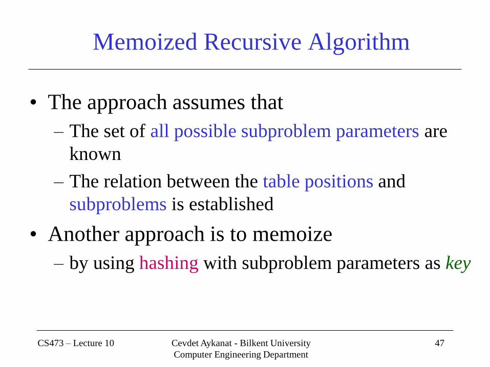
Memoized Recursive Algorithm
• The approach assumes that
– The set of all possible subproblem parameters are
known
– The relation between the table positions and
subproblems is established
• Another approach is to memoize
– by using hashing with subproblem parameters as key

CS473 – Lecture 10 Cevdet Aykanat - Bilkent University
Computer Engineering Department
48
Memoized Recursive Matrix-chain Order
LookupC(p, i, j)
if m[i, j] = then
if i = j then m[i, j] 0
else
for k i to j 1 do
q LookupC(p, i, k) LookupC(p, k1, j) pi-1 pk pj
if q < m[i, j] then
m[i, j] q
return m[i, j]
MemoizedMatrixChain(p)
n length[p] 1
for i 1 to n do
for j 1 to n do
m[i, j]
return LookupC(p, 1, n)
Shaded subtrees are looked-up
rather than recomputing

CS473 – Lecture 10 Cevdet Aykanat - Bilkent University
Computer Engineering Department
49
Elements of Dynamic Programming:
Summary
• Matrix-chain multiplication can be solved in O(n3) time
– by either a top-down memoized recursive algorithm
– or a bottom-up dynamic programming algorithm
• Both methods exploit the overlapping subproblems
property
– There are only (n2) different subproblems in total
– Both methods compute the soln to each problem once
• Without memoization the natural recursive algorithm
runs in exponential time since subproblems are solved
repeatedly

CS473 – Lecture 10 Cevdet Aykanat - Bilkent University
Computer Engineering Department
50
Elements of Dynamic Programming:
Summary
In general practice
• If all subproblems must be solved at once
– a bottom-up DP algorithm always outperforms a top-down memoized algorithm by a constant factor
because, bottom-up DP algorithm
• Has no overhead for recursion
• Less overhead for maintaining the table
• DP: Regular pattern of table accesses can be exploited to reduce the time and/or space requirements even further
• Memoized: If some problems need not be solved at all, it has
the advantage of avoiding solutions to those subproblems

CS473 – Lecture 10 Cevdet Aykanat - Bilkent University
Computer Engineering Department
51
Longest Common Subsequence
A subsequence of a given sequence is just the given sequence
with some elements (possibly none) left out
Formal definition: Given a sequence X x1, x2, …, xm,
sequence Z z1, z2, …, zk is a subsequence of X
if a strictly increasing sequence i1, i2, …, ik of indices of X such that xi zj for all j 1, 2, …, k, where 1 k m
1 2 3 4 5 6 7
Example: Z B,C,D,B is a subsequence of X A,B,C,B,D,A,B
with the index sequence i1, i2, i3, i4 2, 3, 5, 7
CS473 – Lecture 10 Cevdet Aykanat - Bilkent University
Computer Engineering Department
52
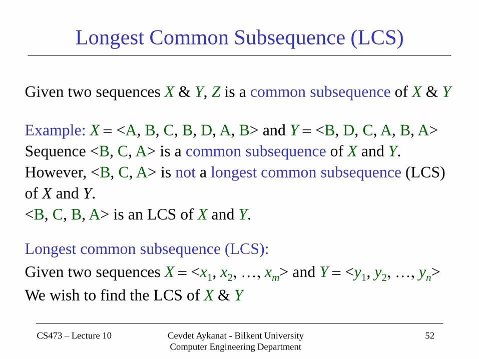
Longest Common Subsequence (LCS)
Given two sequences X & Y, Z is a common subsequence of X & Y
Example: X <A, B, C, B, D, A, B> and Y <B, D, C, A, B, A>
Sequence <B, C, A> is a common subsequence of X and Y.
However, <B, C, A> is not a longest common subsequence (LCS)
of X and Y.
<B, C, B, A> is an LCS of X and Y.
Longest common subsequence (LCS):
Given two sequences X <x1, x2, …, xm> and Y <y1, y2, …, yn>
We wish to find the LCS of X & Y
CS473 – Lecture 10 Cevdet Aykanat - Bilkent University
Computer Engineering Department
53
Characterizing a Longest Common Subsequence
A brute force approach
• Enumerate all subsequences of X
• Check each subsequence to see if it is also a subsequence of Y
meanwhile keeping track of the LCS found
• Each subsequence of X corresponds to a subset of the index
set {1, 2, …, m} of X
• So, there are 2m subsequences of X
• Hence, this approach requires exponential time

CS473 – Lecture 10 Cevdet Aykanat - Bilkent University
Computer Engineering Department
54
Characterizing a Longest Common Subsequence
Definition: The i-th prefix Xi of X for i 0,1, …, m is Xi <x1, x2, …, xi>
1 2 3 4 5 6 7
Example: Given X <A, B, C, B, D, A, B>
X4 <A, B, C, B> and X empty sequence
Theorem: (Optimal substructure of an LCS)
Let X <x1, x2, …, xm> and Y <y1, y2, …, yn> are given
Let Z <z1, z2, …, zk> be any LCS of X and Y
1. If xm yn then zk xm yn and Zk1 is an LCS of Xm1 and Yn1
2. If xm yn and zk xm then Z is an LCS of Xm1 and Y
3. If xm yn and zk yn then Z is an LCS of X and Yn 1
CS473 – Lecture 10 Cevdet Aykanat - Bilkent University
Computer Engineering Department
55
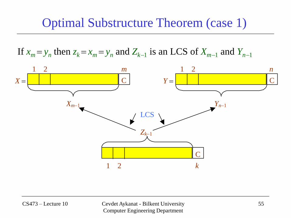
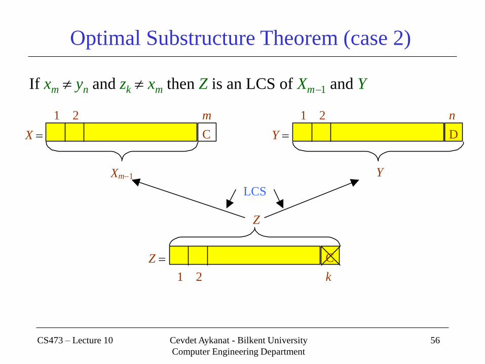
Optimal Substructure Theorem (case 1)
If xm yn then zk xm yn and Zk1 is an LCS of Xm1 and Yn1
Xm1
1 2 m
X C Y
1 2 n
C
Yn1
C
1 2 k
Zk1
LCS
CS473 – Lecture 10 Cevdet Aykanat - Bilkent University
Computer Engineering Department
56
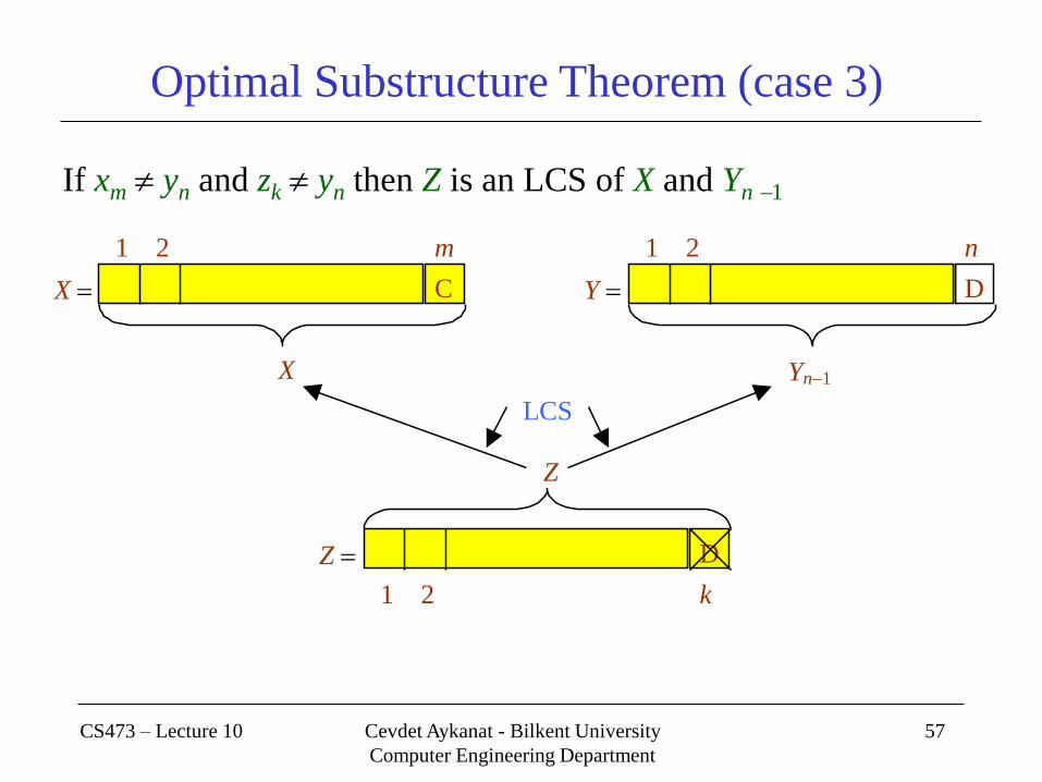
Optimal Substructure Theorem (case 2)
If xm yn and zk xm then Z is an LCS of Xm1 and Y
Xm1
1 2 m
X C Y
1 2 n
D
Y
1 2 k
Z
LCS
Z C
CS473 – Lecture 10 Cevdet Aykanat - Bilkent University
Computer Engineering Department
57
Optimal Substructure Theorem (case 3)
If xm yn and zk yn then Z is an LCS of X and Yn 1
X
1 2 m
X C Y
1 2 n
D
Yn1
D
1 2 k
Z
LCS
Z
CS473 – Lecture 10 Cevdet Aykanat - Bilkent University
Computer Engineering Department
58
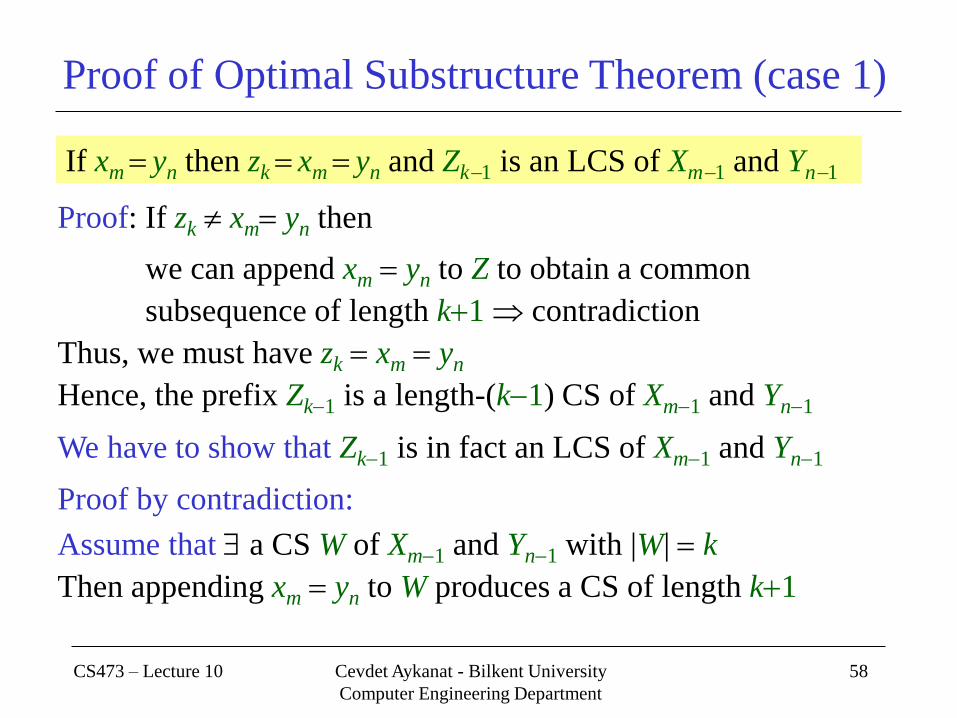
Proof of Optimal Substructure Theorem (case 1)
Proof: If zk xm yn then
we can append xm yn to Z to obtain a common
subsequence of length k1 contradiction
Thus, we must have zk xm yn
Hence, the prefix Zk1 is a length-(k1) CS of Xm1 and Yn1
We have to show that Zk1 is in fact an LCS of Xm1 and Yn1
Proof by contradiction:
Assume that a CS W of Xm1 and Yn1 with |W| k
Then appending xm yn to W produces a CS of length k1
If xm yn then zk xm yn and Zk1 is an LCS of Xm1 and Yn1

CS473 – Lecture 10 Cevdet Aykanat - Bilkent University
Computer Engineering Department
59
Proof of Optimal Substructure Theorem (case 2)
Proof : If zk xm then Z is a CS of Xm1 and Yn
We have to show that Z is in fact an LCS of Xm1 and Yn
(Proof by contradiction)
Assume that a CS W of Xm1 and Yn with |W| > k
Then W would also be a CS of X and Y
Contradiction to the assumption that
Z is an LCS of X and Y with |Z| k
Case 3: Dual of the proof for (case 2)
If xm yn and zk xm then Z is an LCS of Xm1 and Y

CS473 – Lecture 10 Cevdet Aykanat - Bilkent University
Computer Engineering Department
60
Longest Common Subsequence Algorithm
LCS(X, Y)
m length[X]
n length[Y]
if xm yn then
Z LCS(Xm1, Yn1) solve one subproblem
return <Z, xm yn> append xm yn to Z
else
Z LCS(Xm1, Y)
Z LCS(X, Yn1)
return longer of Z and Z
solve two subproblems
CS473 – Lecture 10 Cevdet Aykanat - Bilkent University
Computer Engineering Department
61
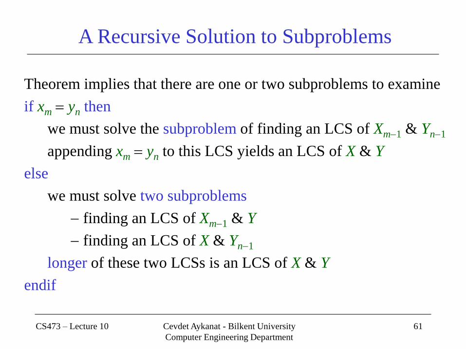
A Recursive Solution to Subproblems
Theorem implies that there are one or two subproblems to examine
if xm yn then
we must solve the subproblem of finding an LCS of Xm1 & Yn1
appending xm yn to this LCS yields an LCS of X & Y
else
we must solve two subproblems
finding an LCS of Xm1 & Y
finding an LCS of X & Yn1
longer of these two LCSs is an LCS of X & Y
endif

CS473 – Lecture 10 Cevdet Aykanat - Bilkent University
Computer Engineering Department
62
A Recursive Solution to Subproblems
Overlapping-subproblems property
finding an LCS to Xm1 & Y and an LCS to X & Yn1 has the subsubproblem of finding an LCS to Xm1 & Yn1
many other subproblems share subsubproblems
A recurrence for the cost of an optimal solution
c[i, j]: length of an LCS of the prefix subsequences Xi & Yj
If either i 0 or j 0, one of the prefix sequences has length 0, so the LCS has length 0
ji
ji
yxji
yxji
ji
jicjic
jicjic
and 0, if
and 0, if
0or 0 if
]},1[],1,[max{
1]1,1[
0
],[

CS473 – Lecture 10 Cevdet Aykanat - Bilkent University
Computer Engineering Department
63
Computing the Length of an LCS
We can easily write an exponential-time recursive algorithm
based on the given recurrence
However, there are only (mn) distinct subproblems
Therefore, we can use dynamic programming
Data structures:
Table c[0…m, 0…n] is used to store c[i, j] values
Entries of this table are computed in row-major order
Table b[1…m, 1…n] is maintained to simplify the construction of an optimal solution
b[i, j]: points to the table entry corresponding to the optimal subproblem solution chosen when computing c[i, j]

CS473 – Lecture 10 Cevdet Aykanat - Bilkent University
Computer Engineering Department
64
Computing the Length of an LCS LCS-LENGTH(X,Y)
m length[X]; n length[Y] for i 0 to m do c[i, 0] 0 for j 0 to n do c[0, j] 0 for i 1 to m do
for j 1 to n do if xi yj then
c[i, j] c[i1, j1]1
b[i, j] “” else if c[i 1, j] c[i, j1]
c[i, j] c[i1, j] b[i, j] “”
else c[i, j] c[i, j1]
b[i, j] “”
CS473 – Lecture 10 Cevdet Aykanat - Bilkent University
Computer Engineering Department
65
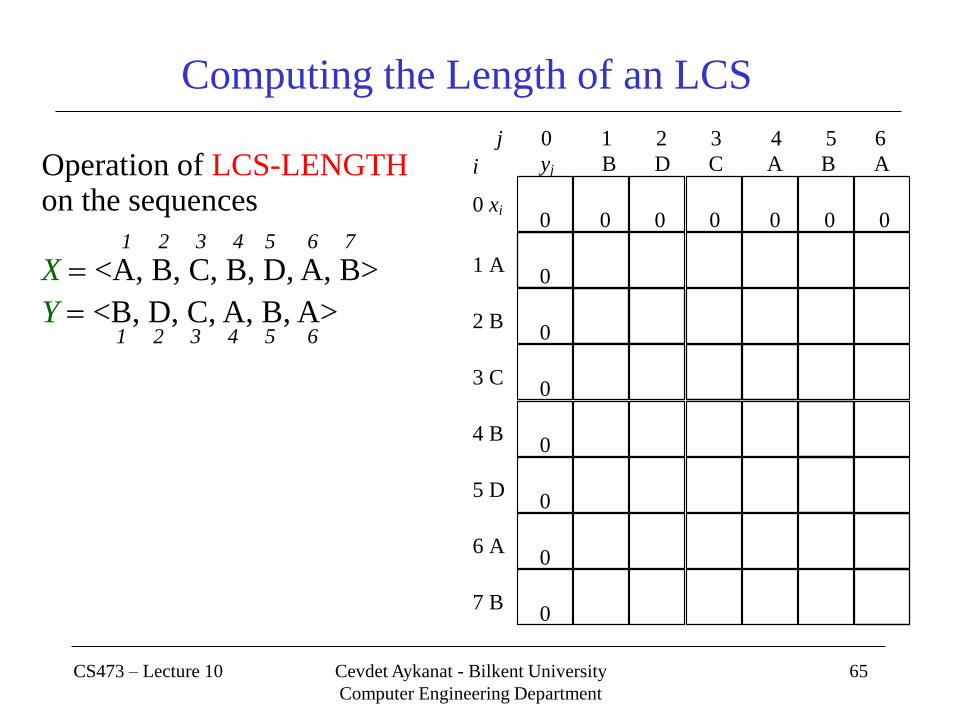
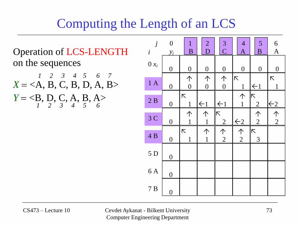
Computing the Length of an LCS
Operation of LCS-LENGTH on the sequences
1 2 3 4 5 6 7
X <A, B, C, B, D, A, B>
Y <B, D, C, A, B, A> 1 2 3 4 5 6
0
0
0
0
0
0
0
0 0 0 0 0 0 0
j 0 1 2 3 4 5 6
yj B D C A B A i
0 xi
1 A
2 B
3 C
4 B
5 D
6 A
7 B
CS473 – Lecture 10 Cevdet Aykanat - Bilkent University
Computer Engineering Department
66
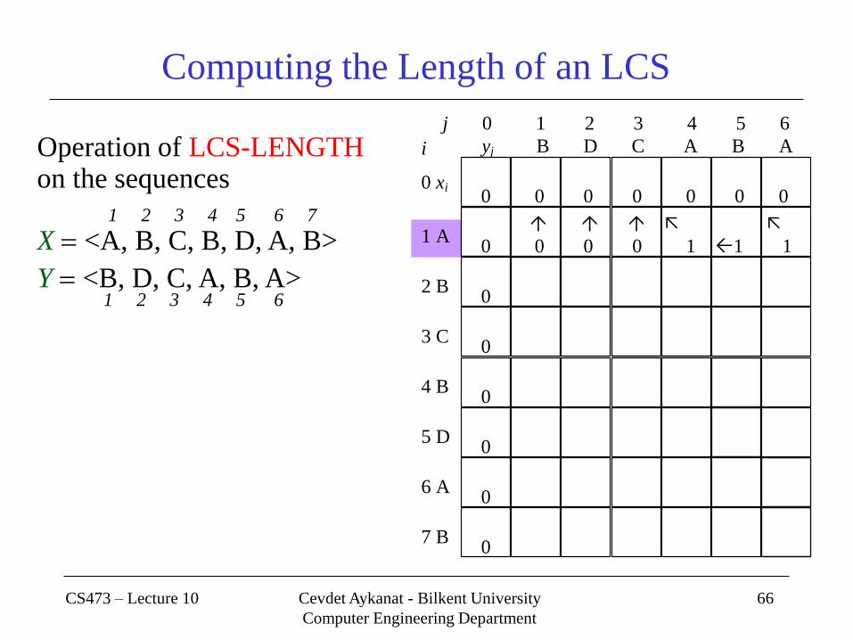
Computing the Length of an LCS
Operation of LCS-LENGTH on the sequences
1 2 3 4 5 6 7
X <A, B, C, B, D, A, B>
Y <B, D, C, A, B, A> 1 2 3 4 5 6
1 A
0
0 0 0 0 1 1 1
0
0
0
0
0
0 0 0 0 0 0 0
j 0 1 2 3 4 5 6
yj B D C A B A i
0 xi
2 B
3 C
4 B
5 D
6 A
7 B

CS473 – Lecture 10 Cevdet Aykanat - Bilkent University
Computer Engineering Department
67
Computing the Length of an LCS
Operation of LCS-LENGTH on the sequences
1 2 3 4 5 6 7
X <A, B, C, B, D, A, B>
Y <B, D, C, A, B, A> 1 2 3 4 5 6
0
0 0 0 0 1 1 1
0 1 1 1 1 2 2
0
0
0
0
j 0 1 2 3 4 5 6
yj B D C A B A
0 0 0 0 0 0 0
i
0 xi
1 A
2 B
3 C
4 B
5 D
6 A
7 B
CS473 – Lecture 10 Cevdet Aykanat - Bilkent University
Computer Engineering Department
68
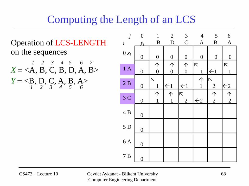
Computing the Length of an LCS
Operation of LCS-LENGTH on the sequences
1 2 3 4 5 6 7
X <A, B, C, B, D, A, B>
Y <B, D, C, A, B, A> 1 2 3 4 5 6
0
0 0 0 0 1 1 1
0 1 1 1 1 2 2
0 1 1 2 2 2 2
0
0
0
j 0 1 2 3 4 5 6
yj B D C A B A
0 0 0 0 0 0 0
i
0 xi
1 A
2 B
3 C
4 B
5 D
6 A
7 B

CS473 – Lecture 10 Cevdet Aykanat - Bilkent University
Computer Engineering Department
69
Computing the Length of an LCS
Operation of LCS-LENGTH on the sequences
1 2 3 4 5 6 7
X <A, B, C, B, D, A, B>
Y <B, D, C, A, B, A> 1 2 3 4 5 6
0
0 0 0 0 0 0 0
0 0 0 0 1 1 1
0 1 1 1 1 2 2
0 1 1 2 2 2 2
0 1
0
0
j 0 1 2 3 4 5 6
yj B D C A B A i
0 xi
1 A
2 B
3 C
4 B
5 D
6 A
7 B

CS473 – Lecture 10 Cevdet Aykanat - Bilkent University
Computer Engineering Department
70
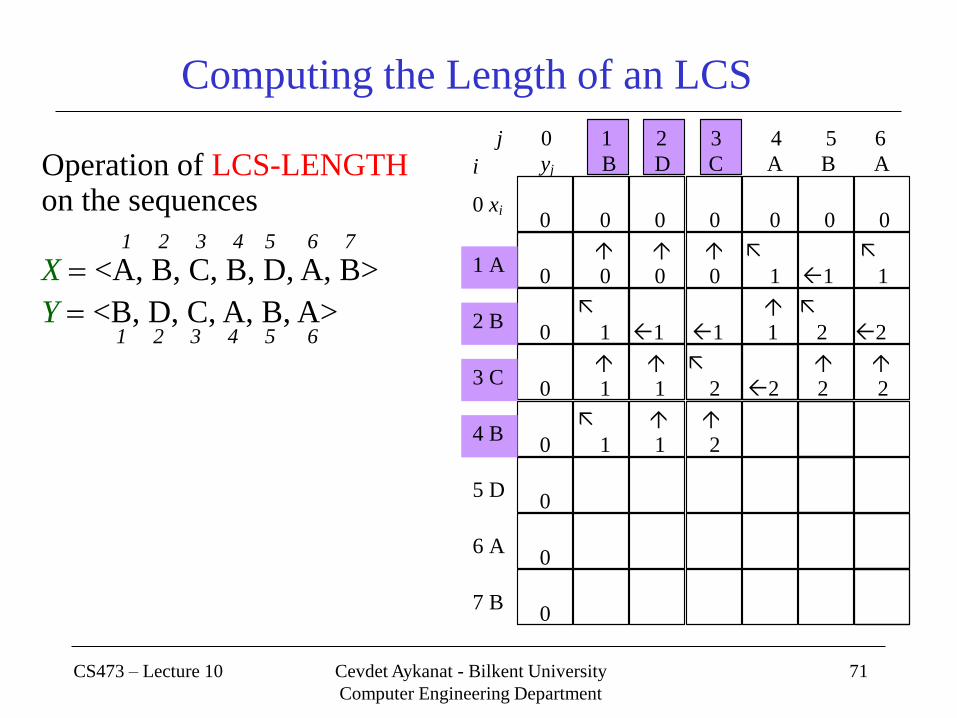
Computing the Length of an LCS
Operation of LCS-LENGTH on the sequences
1 2 3 4 5 6 7
X <A, B, C, B, D, A, B>
Y <B, D, C, A, B, A> 1 2 3 4 5 6
0
0 0 0 0 0 0 0
0 0 0 0 1 1 1
0 1 1 1 1 2 2
0 1 1 2 2 2 2
0 1 1
0
0
j 0 1 2 3 4 5 6
yj B D C A B A i
0 xi
1 A
2 B
3 C
4 B
5 D
6 A
7 B
CS473 – Lecture 10 Cevdet Aykanat - Bilkent University
Computer Engineering Department
71
Computing the Length of an LCS
Operation of LCS-LENGTH on the sequences
1 2 3 4 5 6 7
X <A, B, C, B, D, A, B>
Y <B, D, C, A, B, A> 1 2 3 4 5 6
0
0 0 0 0 0 0 0
0 0 0 0 1 1 1
0 1 1 1 1 2 2
0 1 1 2 2 2 2
0 1 1 2
0
0
j 0 1 2 3 4 5 6
yj B D C A B A i
0 xi
1 A
2 B
3 C
4 B
5 D
6 A
7 B

CS473 – Lecture 10 Cevdet Aykanat - Bilkent University
Computer Engineering Department
72
Computing the Length of an LCS
Operation of LCS-LENGTH on the sequences
1 2 3 4 5 6 7
X <A, B, C, B, D, A, B>
Y <B, D, C, A, B, A> 1 2 3 4 5 6
0
0 0 0 0 0 0 0
0 0 0 0 1 1 1
0 1 1 1 1 2 2
0 1 1 2 2 2 2
0 1 1 2 2
0
0
j 0 1 2 3 4 5 6
yj B D C A B A i
0 xi
1 A
2 B
3 C
4 B
5 D
6 A
7 B
CS473 – Lecture 10 Cevdet Aykanat - Bilkent University
Computer Engineering Department
73
Computing the Length of an LCS
Operation of LCS-LENGTH on the sequences
1 2 3 4 5 6 7
X <A, B, C, B, D, A, B>
Y <B, D, C, A, B, A> 1 2 3 4 5 6
0
0 0 0 0 0 0 0
0 0 0 0 1 1 1
0 1 1 1 1 2 2
0 1 1 2 2 2 2
0 1 1 2 2 3
0
0
j 0 1 2 3 4 5 6
yj B D C A B A i
0 xi
1 A
2 B
3 C
4 B
5 D
6 A
7 B

CS473 – Lecture 10 Cevdet Aykanat - Bilkent University
Computer Engineering Department
74
Computing the Length of an LCS
Operation of LCS-LENGTH on the sequences
1 2 3 4 5 6 7
X <A, B, C, B, D, A, B>
Y <B, D, C, A, B, A> 1 2 3 4 5 6
0
0 0 0 0 0 0 0
0 0 0 0 1 1 1
0 1 1 1 1 2 2
0 1 1 2 2 2 2
0 1 1 2 2 3 3
0
0
j 0 1 2 3 4 5 6
yj B D C A B A i
0 xi
1 A
2 B
3 C
4 B
5 D
6 A
7 B

CS473 – Lecture 10 Cevdet Aykanat - Bilkent University
Computer Engineering Department
75
Computing the Length of an LCS
Operation of LCS-LENGTH on the sequences
1 2 3 4 5 6 7
X <A, B, C, B, D, A, B>
Y <B, D, C, A, B, A> 1 2 3 4 5 6
0
0 0 0 0 1 1 1
0 1 1 1 1 2 2
0 1 1 2 2 2 2
0 1 1 2 2 3 3
0 1 2 2 2 3 3
0
j 0 1 2 3 4 5 6
yj B D C A B A
0 0 0 0 0 0 0
i
0 xi
1 A
2 B
3 C
4 B
5 D
6 A
7 B

CS473 – Lecture 10 Cevdet Aykanat - Bilkent University
Computer Engineering Department
76
Computing the Length of an LCS
Operation of LCS-LENGTH on the sequences
1 2 3 4 5 6 7
X <A, B, C, B, D, A, B>
Y <B, D, C, A, B, A> 1 2 3 4 5 6
0
0 0 0 0 1 1 1
0 1 1 1 1 2 2
0 1 1 2 2 2 2
0 1 1 2 2 3 3
0 1 2 2 2 3 3
0 1 2 2 3 3 4
j 0 1 2 3 4 5 6
yj B D C A B A
0 0 0 0 0 0 0
i
0 xi
1 A
2 B
3 C
4 B
5 D
6 A
7 B

CS473 – Lecture 10 Cevdet Aykanat - Bilkent University
Computer Engineering Department
77
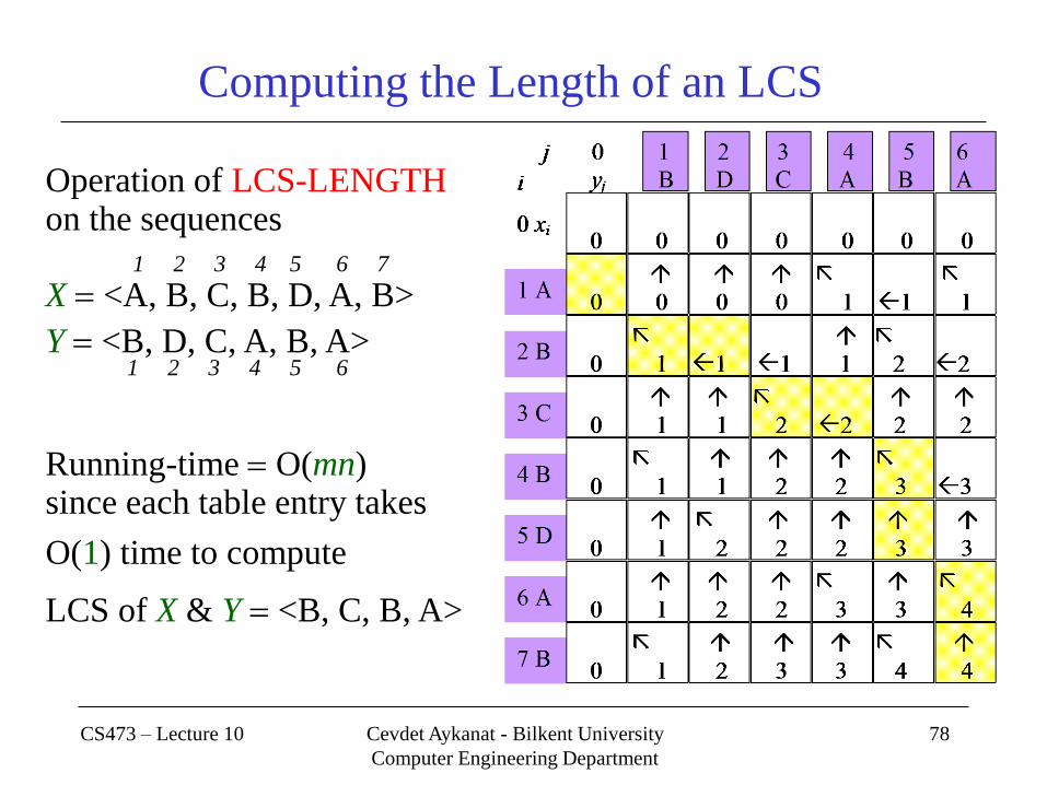
Computing the Length of an LCS
Operation of LCS-LENGTH on the sequences
1 2 3 4 5 6 7
X <A, B, C, B, D, A, B>
Y <B, D, C, A, B, A> 1 2 3 4 5 6
Running-time O(mn) since each table entry takes
O(1) time to compute
LCS of X & Y <B, C, B, A>
0 1 2 3 3 4 4
0 1 1 1 1 2 2
0 1 1 2 2 2 2
0 1 1 2 2 3 3
0 1 2 2 2 3 3
0 1 2 2 3 3 4
0 0 0 0 1 1 1
0 0 0 0 0 0 0
j 0 1 2 3 4 5 6
yj B D C A B A i
0 xi
1 A
2 B
3 C
4 B
5 D
6 A
7 B
CS473 – Lecture 10 Cevdet Aykanat - Bilkent University
Computer Engineering Department
78
Computing the Length of an LCS
Operation of LCS-LENGTH on the sequences
1 2 3 4 5 6 7
X <A, B, C, B, D, A, B>
Y <B, D, C, A, B, A> 1 2 3 4 5 6
Running-time O(mn) since each table entry takes
O(1) time to compute
LCS of X & Y <B, C, B, A>

CS473 – Lecture 10 Cevdet Aykanat - Bilkent University
Computer Engineering Department
79
Constructing an LCS
The b table returned by LCS-LENGTH can be used to quickly
construct an LCS of X & Y
Begin at b[m, n] and trace through the table following arrows
Whenever you encounter a “” in entry b[i, j]
it implies that xi yj is an element of LCS
The elements of LCS are encountered in reverse order
CS473 – Lecture 10 Cevdet Aykanat - Bilkent University
Computer Engineering Department
80
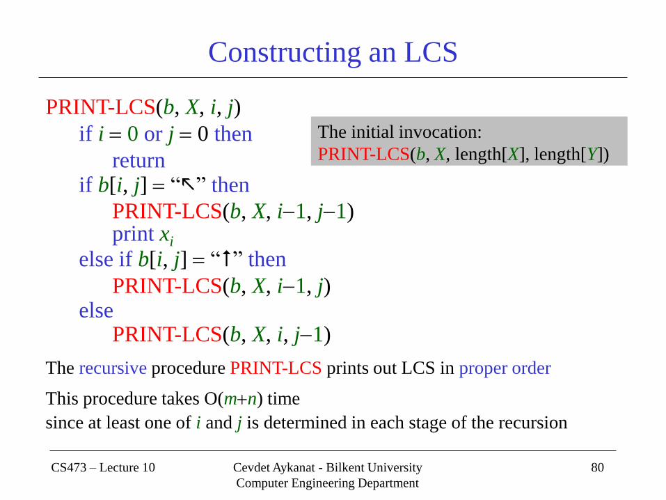
Constructing an LCS
PRINT-LCS(b, X, i, j)
if i 0 or j 0 then
return if b[i, j] “” then
PRINT-LCS(b, X, i1, j1) print xi
else if b[i, j] “” then
PRINT-LCS(b, X, i1, j) else
PRINT-LCS(b, X, i, j1)
The recursive procedure PRINT-LCS prints out LCS in proper order
This procedure takes O(mn) time
since at least one of i and j is determined in each stage of the recursion
The initial invocation:
PRINT-LCS(b, X, length[X], length[Y])

CS473 – Lecture 10 Cevdet Aykanat - Bilkent University
Computer Engineering Department
81
Longest Common Subsequence Improving the code:
we can eliminate the b table altogether
each c[i, j] entry depends only on 3 other c table entries
c[i1, j1], c[i1, j] and c[i, j1]
Given the value of c[i, j]
we can determine in O(1) time which of these 3 values was used
to compute c[i, j] without inspecting table b
we save (mn) space by this method
however, space requirement is still (mn)
since we need (mn) space for the c table anyway
We can reduce the asymptotic space requirement for LCS-LENGTH
since it needs only two rows of table c at a time
the row being computed and the previous row
This improvement works if we only need the length of an LCS


![Java Coding 6 - Bilkent Universitycs.bilkent.edu.tr/~erman/CS101/Set8.pdf · setOfValues –int[] Easy Problem with Methods! •Identify method signatures from algorithm 1. read set](https://static.fdocuments.us/doc/165x107/5e811109791d5d4e6f348725/java-coding-6-bilkent-ermancs101set8pdf-setofvalues-aint-easy-problem.jpg)
![arXiv:1412.8081v1 [q-bio.QM] 27 Dec 2014 · AvoidingtippingpointsinfisheriesmanagementthroughGaussianProcess DynamicProgramming CarlBoettigera,∗,MarcMangela,StephanMunchb aCenterforStockAssessmentResearch](https://static.fdocuments.us/doc/165x107/5ebb5977f2e66f150259fc48/arxiv14128081v1-q-bioqm-27-dec-2014-avoidingtippingpointsinisheriesmanagementthroughgaussianprocess.jpg)