Lecture 1: Traditional Open Macro Models and Monetary · PDF fileEx 1: The Cagan Model Ex 2:...

Ex 1: The Cagan ModelEx 2: Open-economy extension

Ex 3: The Mundell-Fleming-Dornbusch model

Lecture 1: Traditional Open Macro Models andMonetary Policy

Isabelle [email protected]

http://mejean.isabelle.googlepages.com/

Master Economics and Public Policy, International Macroeconomics

October 16th, 2008

Isabelle Mejean Lecture 1



Introduction

Many important questions in international macroeconomics involvemonetary issues

The main departure with respect to a closed economy is that severalmonetary authorities play independently, managing differentcurrencies.

Introducing money in a model allows addressing a number of issues:determinants of seignorage, mechanics of exchange-rate systems,long-run effects of money-supply changes on prices and exchangerates




Introduction (2)

Role of money

i) Medium of exchangeii) Store of valueiii) Nominal unit of account

Nature of money

Here, money is meant as currency (abstract from the bankingsystem)Money does not bear interest ⇒ Simplifying assumption ≈ Liquiditypremium




The Cagan Model




Hypotheses

Simple empirical model of money and inflation used to studyhyperinflations (ie inflation > 50% per month, ex Zimbabwe: 100000% in january 2008)

Prices are fully flexible ⇒ Adjust to clear product, factor and assetmarkets ⇒ Long-run analysis

Stochastic, discrete-time model

Rational expectations




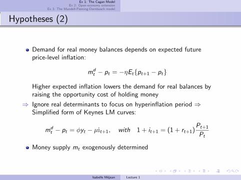
Hypotheses (2)

Demand for real money balances depends on expected futureprice-level inflation:

mdt − pt = −ηEt{pt+1 − pt}

Higher expected inflation lowers the demand for real balances byraising the opportunity cost of holding money

⇒ Ignore real determinants to focus on hyperinflation period ⇒Simplified form of Keynes LM curves:

mdt − pt = φyt − µit+1, with 1 + it+1 = (1 + rt+1)

Pt+1

Pt

Money supply mt exogenously determined




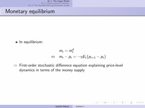
Monetary equilibrium

In equilibrium:

mt = mdt

⇔ mt − pt = −ηEt{pt+1 − pt}

⇒ First-order stochastic difference equation explaining price-leveldynamics in terms of the money supply




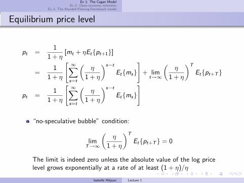
Equilibrium price level

pt =1

1 + η[mt + ηEt{pt+1}]

=1

1 + η

[ ∞∑s=t

(η

1 + η

)s−t

Et{ms}

]+ lim

t→∞

(η

1 + η

)T

Et{pt+T}

pt =1

1 + η

[ ∞∑s=t

(η

1 + η

)s−t

Et{ms}

]

“no-speculative bubble” condition:

limT→∞

(η

1 + η

)T

Et{pt+T} = 0

The limit is indeed zero unless the absolute value of the log pricelevel grows exponentially at a rate of at least (1 + η)/η




Equilibrium price level (2)

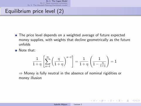
The price level depends on a weighted average of future expectedmoney supplies, with weights that decline geometrically as the futureunfolds

Note that:

1

1 + η

[ ∞∑s=t

(η

1 + η

)s−t]

=1

1 + η

(1

1− η1+η

)= 1

⇒ Money is fully neutral in the absence of nominal rigidities ormoney illusion




Constant money supply

mt = m,∀t

⇒ Zero expected inflation : Etpt+1 − pt = 0,

⇒ Constant price level: p = m




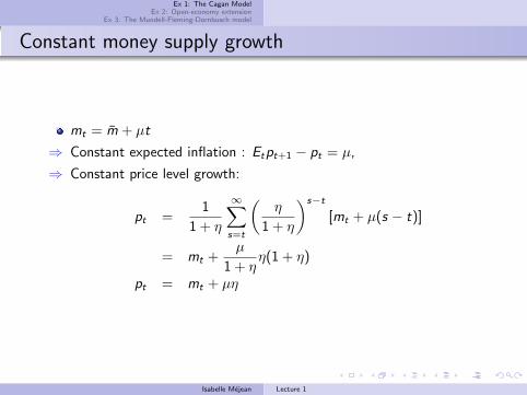
Constant money supply growth

mt = m + µt

⇒ Constant expected inflation : Etpt+1 − pt = µ,

⇒ Constant price level growth:

pt =1

1 + η

∞∑s=t

(η

1 + η

)s−t

[mt + µ(s − t)]

= mt +µ

1 + ηη(1 + η)

pt = mt + µη




Autoregressive money supply

mt = ρmt−1 + εt , 0 ≤ ρ ≤ 1, Et{εt+1} = 0

Price level:

pt =mt

1 + η

∞∑s=t

(ηρ

1 + η

)s−t

=mt

1 + η − ηρ

In the limiting case ρ = 1 in which money shocks are expected to bepermanent, the solution reduces to pt = mt .




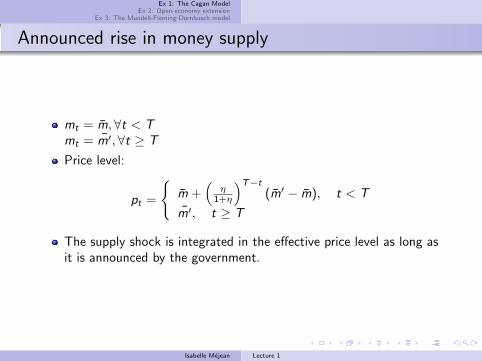
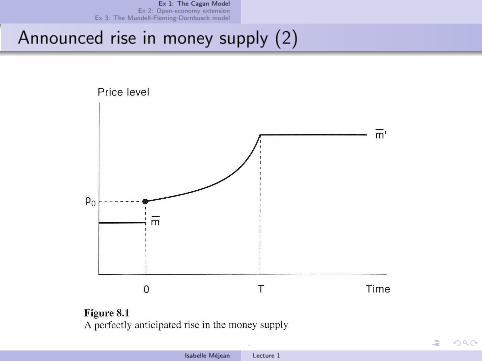
Announced rise in money supply

mt = m,∀t < Tmt = m′,∀t ≥ T

Price level:

pt =

{m +

(η

1+η

)T−t

(m′ − m), t < T

m′, t ≥ T

The supply shock is integrated in the effective price level as long asit is announced by the government.




Announced rise in money supply (2)




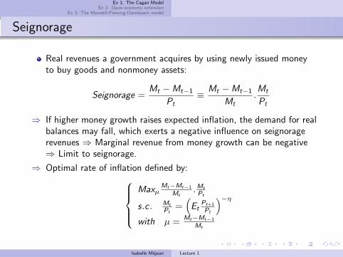
Seignorage

Real revenues a government acquires by using newly issued moneyto buy goods and nonmoney assets:

Seignorage =Mt −Mt−1

Pt≡ Mt −Mt−1

Mt.Mt

Pt

⇒ If higher money growth raises expected inflation, the demand for realbalances may fall, which exerts a negative influence on seignoragerevenues ⇒ Marginal revenue from money growth can be negative⇒ Limit to seignorage.

⇒ Optimal rate of inflation defined by:Maxµ

Mt−Mt−1

Mt.Mt

Pt

s.c . Mt

Pt=(Et

Pt+1

Pt

)−η

with µ = Mt−Mt−1

Mt




Optimal Seignorage under Constant Money Growth

Mt

Mt−1= Pt

Pt−1= 1 + µ

The optimal growth rate of money supply is then:

µ∗ =1

η

Inverse function of the semielasticity of real balances with respect toinflation




How important is seignorage ?

Table: Average 1990-94 seignorage revenues in industrialized countries

Country % Government spending % GDPAustralia 0.95 0.31Canada 0.84 0.09France -0.83 -0.23Germany 2.89 0.56Italy 3.11 0.32New Zealand 0.04 0.01Sweden 3.22 1.52United States 2.19 0.44Source: Obstfeld & Rogoff from IMF-IFS data




Limits

⇒ How can we explain periods of hyperinflation, in which governmentsobviously let money growth exceed the optimal rate?Backward-looking expectations ?

⇒ Credibility issues : On date 0, the government announces that it willstick to the revenue-maximizing rate of money growth → If agentsbelieve it, they hold real balances M/P = [(1 + η)/η]−η → On date1, the government has an incentive to cheat and choose a highermoney growth rate → If governments lack credit, agents willanticipate the government’s temptation to cheat.




Open-economy extensionObstfeld & Rogoff




Hypotheses of the model

Small open economy

Exogenous output

Money demand defined by:

mt − pt = −ηit+1 + φyt

Flexible prices and PPP:

pt = et + p∗t

with et the (log of) nominal exchange rate (home currency per unitof foreign currency) and p∗t the world foreign-currency price




Hypotheses of the model (2)

Uncovered interest parity:

1 + it+1 = (1 + i∗t+1)Et

{Et+1

Et

}⇔ it+1 = i∗t+1 + Etet+1 − et

Simple arbitrage argument under perfect foresight and noexchange-rate risk premium

Note that the log UIP relation is only an approximation since, by theJensen’s inequality, lnEt{Et+1} > Et{ln Et+1}.




Exchange-rate dynamics

Incorporating the PPP and the IUP conditions into the moneydemand gives:

mt − p∗t − et = −ηi∗t+1 − η(Et{et+1} − et) + φyt

⇔ mt − φyt + ηi∗t+1 − p∗t − et = −η(Et{et+1} − et)

Solving for et implies:

et =1

1 + η

∞∑s=t

(η

1 + η

)s−t

Et{ms − φys + ηi∗s+1 − p∗s }




Exchange-rate dynamics (2)

⇒ Describes the behaviour of nominal exchange rates as a function ofexpectations of future variables (≈ asset pricing equations).

Nominal exchange-rate depreciation if:

the path of the home money supply raises, thus increasing thedomestic price level and the exchange rate (through PPP)the real domestic income goes down, thus contracting moneydemand which exerts a negative pressure on the domestic price levelthe foreign interest rate increasesthe foreign price level drops

Note that this equation relies on a PPP assumption ⇒ Long-runModel




Autoregressive money growth

mt −mt−1 = ρ(mt−1 −mt−2) + εt where ε iid, Et−1{εt} = 0

Expected rate of exchange rate depreciation:

Et{et+1} − et =1

1 + η

∞∑s=t

(η

1 + η

)s−t

Et{ms+1 −ms}

Exchange rate level:

et = mt +η

1 + η

∞∑s=t

(η

1 + η

)s−t

Et{ms+1 −ms}

= mt +ηρ

1 + η − ηρ(mt −mt−1)

⇒ Impact of an unanticipated shock to mt : direct exchange rateincrease ( raises the current nominal money supply) + when ρ > 0,increases expectations of future money growth, thereby pushing theexchange rate even higher.




Exchange rate fixing

Fixed exchange rate: et = e and ηi∗ − φy − p∗ = 0

⇒ Fixed money supply: mt = m = e

Fixed exchange rate: et = e and ηi∗ − φy − p∗ 6= 0

⇒ Money supply endogenous, Adjustment to market-driven fluctuationsin i∗

Future fixing at some future date T : et = e,∀t ≥ TIn period T − 1:

mT−1 − φyT−1 + ηi∗T − p∗T−1 − eT−1 = −η(ET−1eT − eT−1) = 0

iT = i∗T + ET−1eT − eT−1 = i∗T

⇒ i adjusts to satisfy the UIP relation. The monetary equilibriumimplies that m also adjusts, whatever the exchange rate level theprivate sector expects ⇒ The announcement is not a well-adaptedsolution for the exchange rate market to converge towards an“equilibrium” value.


Lecture 1: Traditional Open Macro Models and Monetary · PDF fileEx 1: The Cagan Model Ex 2:...

Documents

Transcript of Lecture 1: Traditional Open Macro Models and Monetary · PDF fileEx 1: The Cagan Model Ex 2:...