Lecture 1 Roadmap, Contents, Basic Concepts Kerschbamer: Imperfectly Competitive Markets.
43
Lecture 1 Roadmap, Contents, Basic Concepts Kerschbamer: Imperfectly Competitive Markets
-
date post
21-Dec-2015 -
Category
Documents
-
view
223 -
download
1
Transcript of Lecture 1 Roadmap, Contents, Basic Concepts Kerschbamer: Imperfectly Competitive Markets.

Lecture 1Roadmap, Contents, Basic Concepts
Kerschbamer: Imperfectly Competitive Markets

2
Scenarios that Yield “Imperfectly Competitive Outcomes”
There are at least three scenarios in which markets yield “non-competitive outcomes”:
• there is a single dominant firm in the market (the monopoly case)
• there is more than one firm in the market, but market conditions (number of firms, degree of product differentiation, type of competition . . . ) are such that “imperfectlycompetitive outcomes” result from “normal competition”, even when no individualfirm is dominant (the standard oligopoly case)
• there is more than one firm in the market, market conditions are such that (eitherperfectly or imperfectly) competitive outcomes result from normal competition,but firms take actions that undermine “normal competition” and help them to getoutcomes that (in the limit) resemble those reached by a single dominant firm (“impeded competition”: cartel formation, explicit or tacit collusion, horizontal or vertical mergers, entry deterrence, etc.)
In this lecture series we look at each of those three cases in turn.
Lecture 1: Roadmap, Contents, Basic Concepts
I The Monopoly Case
This case is interesting and relevant in its own (for instance, Alitalia has a monopoly
on flights from Turin to Milan, while Air France has a monopoly on flights from
Toulouse to Paris) and it is an important building block for the other two parts:
For instance, acting like a multi-product monopolist is the best that can be reached by
collusion. Thus, comparing the multi-product monopoly outcome with the outcome
of “normal competition” yields important insights in
• incentives for firms in the market to collude
• consequences of collusion for consumers
Also, acting like a multi-stage monopolist is an outcome that can be reached by a
vertical merger between two adjacent monopolies. Thus, comparing the multi-stage
monopoly outcome with the outcome of “normal competition” yields important
insights in
• incentives for vertically adjacent firms to merge
• consequences of vertical mergers for consumers
Lecture 1: Roadmap, Contents, Basic Concepts 3
I The Monopoly Case (Cont.)
An important real-world relevant topic in the monopoly part is price-discrimination.
Although price-discrimination is not necessarily welfare decreasing, it has repeatedly
been in the focus of competition policy (probably because it is a sign of market power).
We will first look at the “classical” forms of price discrimination, covering
• first-degree price discrimination
• second-degree price discrimination
• third-degree price discrimination
• bundling and tying
Then we will look at intertemporal price-discrimination covering both
• cases where intertemporal price-discrimination hurts the monopolist (Coase conjecture)
and
• cases where intertemporal price-discrimination allows the monopolist to increase her
profit above the normal monopoly profit
Lecture 1: Roadmap, Contents, Basic Concepts 4

II Oligopoly
In the oligopoly part we start with a particularly implausible framework:
• two firms (duopoly)
• one homogeneous good
• many price-taking consumers
• no fixed costs
• no capacity constraints
• same constant marginal cost for both firms (symmetry)
In this simple framework, we analyze the four basic forms of oligopolistic competition
• Cournot competition
• Bertrand competition
• Stackelberg-Cournot competition
• Stackelberg-Bertrand competition
The main point here is how these four basic oligopoly games differ in their rules of the
market game.
Lecture 1: Roadmap, Contents, Basic Concepts 5
II Oligopoly (Cont.)
Next we lift the unrealistic assumptions one after the other in order to see how market
outcomes change
• in the type of competition (price or quantity)
• in the number of firms (form the small to the large number case)
• in the degree of differentiation (from almost perfect substitutes to almost perfect
complements)
• in the tightness of capacity constraints
• in the “degree of asymmetry” between firms
• . . .
Some of the questions we plan to address are
• Is competition always better for consumers than monopoly?
• Relatedly: Are more firms in the market always better for consumers than less firms?
• Is price competition always better for consumers than quantity competition?
• In a leader follower oligopoly game: Is the leader or the follower better off?
• How does the degree of differentiation affect market prices?
Lecture 1: Roadmap, Contents, Basic Concepts 6
III Impeded Competition
Here (again) we start with a(n) (unrealistic) framework by assuming that firms are able to
write enforceable cartel agreements.
First we ask the question, if firms could write enforceable cartel agreements, and if all firms
join a cartel, what would their market strategy be?
Then we turn to the question whether firms would be willing to join an all-inclusive cartel
(if they could write enforceable cartel agreements), and if not, what would the condition for
cartel stability be?
Then we turn to a more realistic scenario, where cartel agreements are not enforceable
(because they violate competition laws and are therefore not enforced in courts of law)
The first question of interest is, if no external enforcement is available, how can firms be
prevented from deviating from a (competition-hampering) agreement?
A possible answer is: If the same firms compete repeatedly on the same market, they might
be able to reach a collusive outcome by making their behavior today dependent on the
performance of the competitors yesterday.
Lecture 1: Roadmap, Contents, Basic Concepts 7

III Impeded Competition (Cont. 1)
Then we look deeper in the economics of (explicit or tacit) collusion.
A main question in this part of the lecture is, which characteristic of an industry affect
the sustainability of collusion?
We look at supply side factors as
• type of competition (Bertrand vs. Cournot)
• number of competitors in the market
• barriers to entry
• frequency of interaction
• degree of asymmetry between competitors
• prospect of innovation
as well as on demand side factors as
• demand dynamics (growing/stagnating/declining demand)
• demand fluctuations (stable vs. fluctuating demand)
• observability of demand shocks (market transparency)
Lecture 1: Roadmap, Contents, Basic Concepts 8
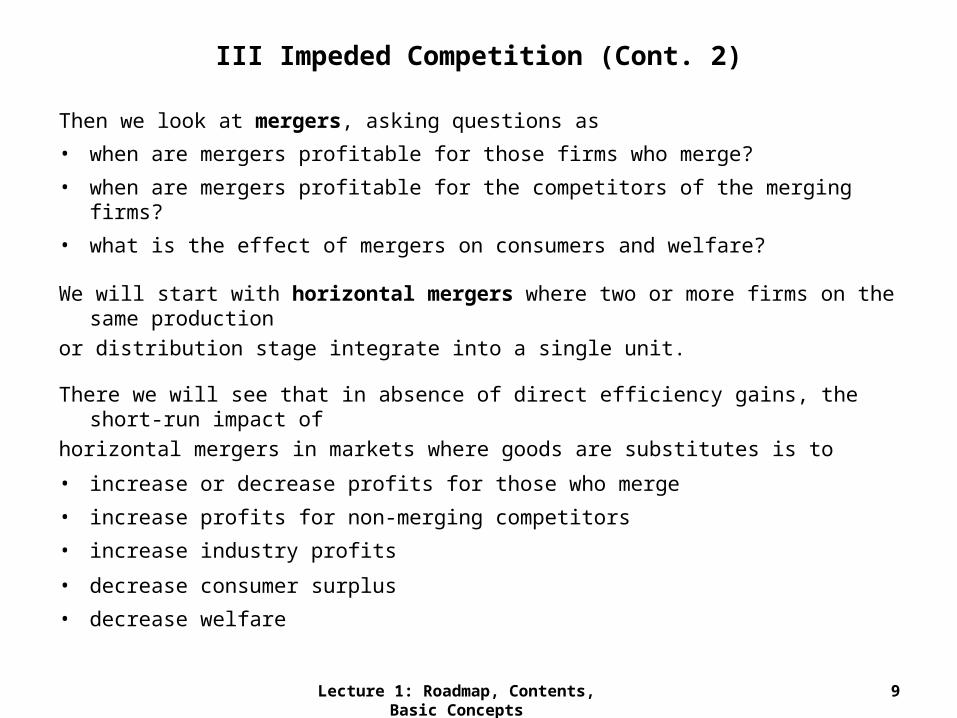
III Impeded Competition (Cont. 2)
Then we look at mergers, asking questions as
• when are mergers profitable for those firms who merge?
• when are mergers profitable for the competitors of the merging firms?
• what is the effect of mergers on consumers and welfare?
We will start with horizontal mergers where two or more firms on the same production
or distribution stage integrate into a single unit.
There we will see that in absence of direct efficiency gains, the short-run impact of
horizontal mergers in markets where goods are substitutes is to
• increase or decrease profits for those who merge
• increase profits for non-merging competitors
• increase industry profits
• decrease consumer surplus
• decrease welfare
Lecture 1: Roadmap, Contents, Basic Concepts 9

III Impeded Competition (Cont. 3)
But, many real worlds mergers involve some form of efficiency gain; and efficiency gains
tend to
• increase profits for those who merge
• decrease the profits for non-merging competitors
• increase industry profits
• increase consumer surplus
• increase welfare
Thus, the desirability of horizontal mergers in markets where goods are substitutes depends
on the magnitude of efficiency gains.
Then we turn to vertical mergers where two or more firms or complementary production
or sales stages integrate into a single unit.
Various effects of vertical mergers have been discussed in the theoretical literature..
Lecture 1: Roadmap, Contents, Basic Concepts 10

III Impeded Competition (Cont. 4)
Various effects of vertical mergers will be discussed
Possible positive effects of vertical mergers include
• avoiding multiple marginalization problems
• avoiding or reducing other vertical externalities
• avoiding “hold ups” and promoting idiosyncratic investments
• avoiding mis-syncronizations
Possible negative effects of vertical mergers include
• increasing market power
• enabling exclusionary behavior
• distorting input choices
If there is time left, we will then turn to other important topics in competition policy as
• entry deterrence (limit pricing)
• exit inducement (predation)
Before we start, we discuss some “technical issues” and some basic concepts that will
be used in different parts of this lecture series. 11

Contents
Part 0: Basic Concepts (Lecture 1)
1. Basics: Quasilinear Preferences and Product Differentiation
1.1 Quasilinear Preferences
1.2 Heterogeneous Goods
• Representative Consumer Models
– Model of Dixit (1979)
• Vertical Product Differentiation
– Model of Shaked and Suttons (1982) [“v(q, θ)= qθ”]
• Horizontal Product Differentiation
– Hotelling (1929)’s Model [“Linear City”]
– Model of D’Aspremont et al. (1979) [“(Linear City)²”]
– Salop (1979)’s Model [“Circular City”]
Lecture 1: Roadmap, Contents, Basic Concepts 12

Contents (Cont. 1)
Part I: Monopoly
2. Dominant but Non-Discriminating Firms (Lecture 2)
• Textbook Monopoly
• Social Loss of Monopoly
• Multiproduct Monopoly
• Multistage Monopoly (Double Marginalization)
3. The Price Discriminating Monopoly (3 Lectures: Lectures 3-5)
• First Degree Price Discrimination
• Second Degree Price Discrimination
– with a Single Two-Part Tariff
– with a Menu of Two-Part Tariffs
– Optimal Second-Degree Price Discrimination
• Third Degree Price Discrimination
• Bundling
• Intertemporal Price Discrimination
Lecture 1: Roadmap, Contents, Basic Concepts 13

Contents (Cont. 2)
Part II: Oligopolistic Competition
4. Oligopolistic Competition (4 Lectures: Lectures 6-9)
• Homogeneous Goods and the Four Market Games
– Cournot Competition
– Bertrand Competition
– Stackelberg-Cournot Competition
– Stackelberg-Bertrand Competition
• Increasing the Number of Competitors
• The Effects of Barriers to Entry
• The Effects of Capacity Constraints
• The Role of Product Differentiation
• Type of Competition and Market Outcomes
• (Product Differentiation) x (Type of Competition)
– Market Demand/Inverse Demand
– Cournot Competition
– Bertrand Competition
– Stackelberg-Cournot Competition
– Stackelberg-Bertrand Competition 14
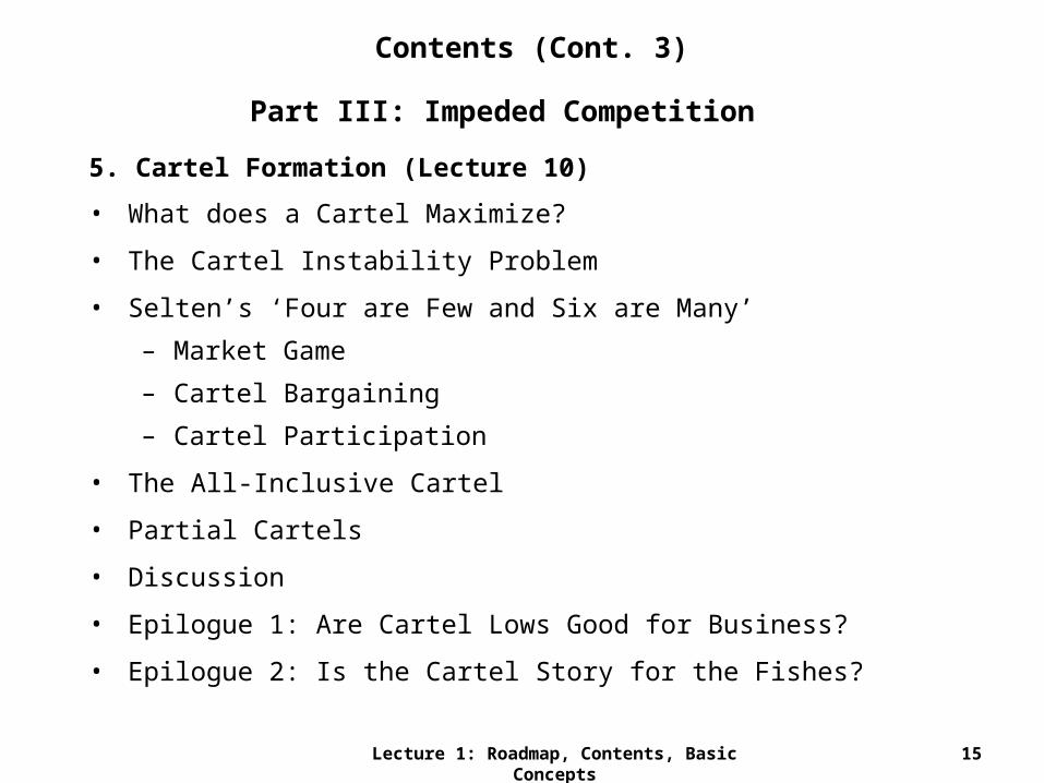
Contents (Cont. 3)
Part III: Impeded Competition
5. Cartel Formation (Lecture 10)
• What does a Cartel Maximize?
• The Cartel Instability Problem
• Selten’s ‘Four are Few and Six are Many’
– Market Game
– Cartel Bargaining
– Cartel Participation
• The All-Inclusive Cartel
• Partial Cartels
• Discussion
• Epilogue 1: Are Cartel Lows Good for Business?
• Epilogue 2: Is the Cartel Story for the Fishes?
Lecture 1: Roadmap, Contents, Basic Concepts 15
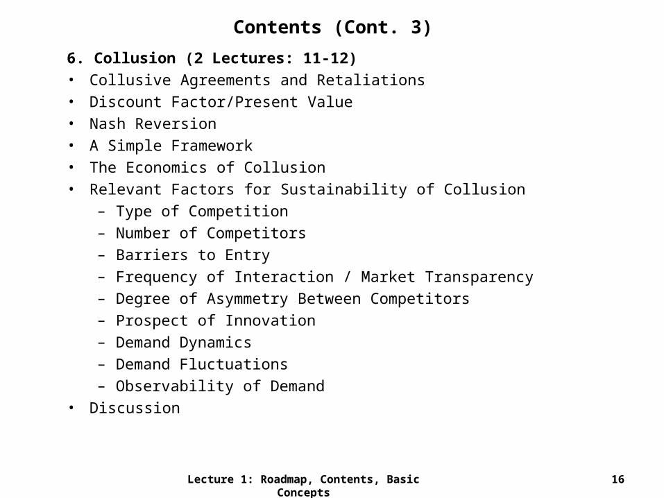
Contents (Cont. 3)
6. Collusion (2 Lectures: 11-12)
• Collusive Agreements and Retaliations
• Discount Factor/Present Value
• Nash Reversion
• A Simple Framework
• The Economics of Collusion
• Relevant Factors for Sustainability of Collusion
– Type of Competition
– Number of Competitors
– Barriers to Entry
– Frequency of Interaction / Market Transparency
– Degree of Asymmetry Between Competitors
– Prospect of Innovation
– Demand Dynamics
– Demand Fluctuations
– Observability of Demand
• Discussion
Lecture 1: Roadmap, Contents, Basic Concepts 16

Contents (Cont. 4)
7. Mergers (2 Lectures: 13-14)
• Horizontal Mergers
– Horizontal Mergers and Market Power
– Horizontal Mergers and Efficiency Gains
– Horizontal Mergers and Structural Effects
• Vertical Mergers
– Vertical Mergers and Pro-competitive Effects
– Vertical Mergers and Anti-competitive Effects
8. Predation and Limit Pricing (if time left)
• exit inducement
• entry deterrence
Lecture 1: Roadmap, Contents, Basic Concepts 17

“Technical Issues”: Partial Equilibrium Analysis
Standard Microeconomics’ main focus is on “general equilibrium”.
In a general equilibrium model “everything depends on everything”: a change in the price of
potatoes might result in changes everywhere in the economy inclusive the demand for red
pens.
This is too complicated for our purposes; we will therefore take a “partial equilibrium”
perspective.
The partial equilibrium approach envisions the market for a single good (or a group of goods)
for which each consumer’s expenditure constitutes only a small portion of his overall budget.
When this is the case, it is reasonable to assume that
• only a small fraction of any increase in wealth will be spent on the market for this good
(those goods) ⇨ wealth effects should be small (really?)
• changes in the market for this good (those goods) will lead to small changes (in prices) in
the rest of the economy ⇨ cross-price effects between this market and the rest of the
economy should be small (really?) Lecture 1: Roadmap, Contents, Basic Concepts 18

Partial Equilibrium Analysis (Cont.)
Throughout this lecture series we take those two conditions not only as given, we rather
assume (these are the ‘partial equilibrium assumptions’):
• that wealth effects are not only small, but absent; and
• that cross-price effects between the market(s) under consideration and the rest of the
economy are not only small but absent.
The fixity of prices of all other goods justifies treating the expenditure on those other goods
as a single composite commodity, called the numeraire.
The absence of wealth effects justifies looking at consumer preferences that are quasilinear
with respect to the numeraire commodity.
Suppose there are two commodities, good X and the numeraire, good Y. Let xi ∈ ℝ+ and
yi (-∞, ∞) denote consumer ∈ i’s consumption of goods X and Y respectively.
Definition. Consumer i’s preference relation on bundles of good X and good Y in
ℝ+ x (-∞, ∞) is quasilinear with respect to good Y if
• all the indifference sets are parallel displacements of each other along the axis of good Y;
• good Y is desirable.Lecture 1: Roadmap, Contents, Basic Concepts 19

Quasilinearity
Definition. Consumer i’s preference relation on bundles of good X and good Y in
ℝ+ x (-∞, ∞) is quasilinear with respect to good Y if
• all the indifference sets are parallel displacements of each other along the axis of good Y;• good Y is desirable.
Note that the definition assumes that there is no lower bound on the possible consumption of
the numeraire commodity. Why is this convenient?
Also note that quasilinear preferences have the property that the consumer’s entire preference
relation can be deducted from a single indifference set.
20
Quasilinear Preferences (w.r.t. good Y)
FIGURE HERE: 1

Quasilinearity (Cont. 1)
Result. A continuous preference relation ≿ on ℝ+ x (-∞, ∞) is quasilinear w.r.t. the
second commodity if and only if it admits a utility function of the form vi(xi,yi) = ui(xi) + yi.
Proof. Omitted – see any advanced micro textbook. ■
In terms of our partial equilibrium interpretation, we think of good X as the good whose
market is under study and of the numeraire as representing the composite of all other goods
In this interpretation, yi stands for the total money expenditure on these other goods.
Throughout, we normalize the price of the numeraire to 1 and we let p denote the price of
good X. The following assumptions on ui(xi) turn out to be useful
• ui(.) is bounded above and twice differentiable
• 0 < ui’(0) < ∞
• ∃ xmax such that ui’(xi) > 0 and ui’’(xi) < 0 for all xi (0, ∈ ximax) and ui‘(xi) = 0 for xi ≥ xi
max
• ui(0) = 0
Lecture 1: Roadmap, Contents, Basic Concepts 21

Quasilinearity (Cont. 2): An Example
Note that with those assumption ui(xi) can be interpreted as consumer i’s willingness
to pay for xi units!
Lecture 1: Roadmap, Contents, Basic Concepts 22
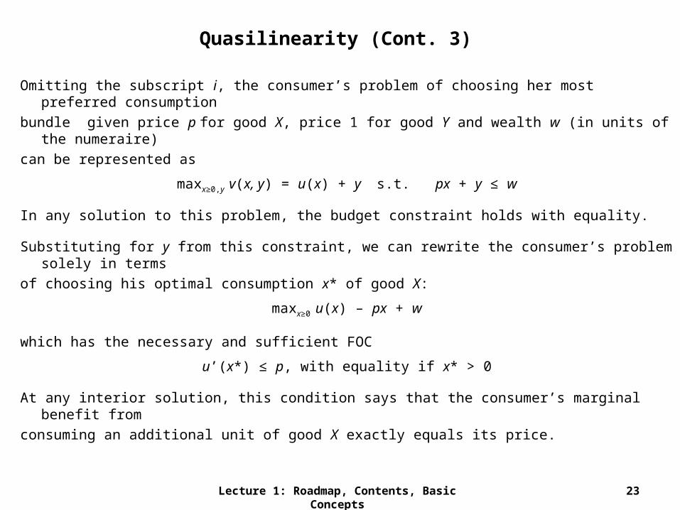
Quasilinearity (Cont. 3)
Omitting the subscript i, the consumer’s problem of choosing her most preferred consumption
bundle given price p for good X, price 1 for good Y and wealth w (in units of the numeraire)
can be represented as
maxx≥0,y v(x, y) = u(x) + y s.t. px + y ≤ w
In any solution to this problem, the budget constraint holds with equality.
Substituting for y from this constraint, we can rewrite the consumer’s problem solely in terms
of choosing his optimal consumption x* of good X:
maxx≥0 u(x) – px + w
which has the necessary and sufficient FOC
u’(x*) ≤ p, with equality if x* > 0
At any interior solution, this condition says that the consumer’s marginal benefit from
consuming an additional unit of good X exactly equals its price.
Lecture 1: Roadmap, Contents, Basic Concepts 23

Quasilinearity (Cont. 4): Deriving Demand
Lecture 1: Roadmap, Contents, Basic Concepts 24
FIGURE HERE: 5 FIGURE HERE: 4
Quasilinearity (Cont. 5)
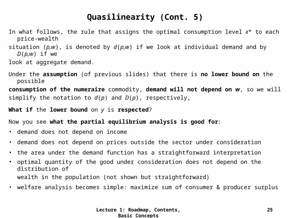
In what follows, the rule that assigns the optimal consumption level x* to each price-wealth
situation (p,w), is denoted by d(p,w) if we look at individual demand and by D(p,w) if we
look at aggregate demand.
Under the assumption (of previous slides) that there is no lower bound on the possible
consumption of the numeraire commodity, demand will not depend on w, so we will
simplify the notation to d(p) and D(p), respectively,
What if the lower bound on y is respected?
Now you see what the partial equilibrium analysis is good for:
• demand does not depend on income
• demand does not depend on prices outside the sector under consideration
• the area under the demand function has a straightforward interpretation
• optimal quantity of the good under consideration does not depend on the distribution of
wealth in the population (not shown but straightforward)
• welfare analysis becomes simple: maximize sum of consumer & producer surplus
Lecture 1: Roadmap, Contents, Basic Concepts 25

Quasilinearity and Heterogeneity of Goods
Much of this lecture series will focus on industries where goods are heterogeneous.
The quasilinear framework can easily be extended to allow for more that one non-
numeraire good.
In what follows we consider a single representative consumer (we can therefore drop the i
subscript) who decides about the quantities x1, . . . , xm of the goods X1, . . . , Xm (note the
misuse of notation; the subscript denotes the good now).
The preferences of the consumer are represented by the quasilinear utility function
v(x1, . . . , xm, y) = u(x1, . . . , xm) + y with
u(x1, . . . , xm) = 0 for x1 = x2 = . . . = xm = 0
Note that u(x1, . . . , xm) can be interpreted as the representative consumer’s willingness to
pay for a bundle containing x1 units of good X1, x2 units of X2, . . .
Similarly ∂u(x1, . . . , xm)/∂xj is the marginal . . .
Lecture 1: Roadmap, Contents, Basic Concepts 26
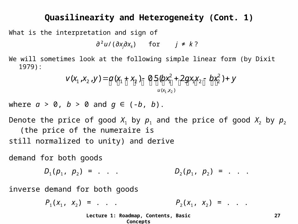
Quasilinearity and Heterogeneity (Cont. 1)
What is the interpretation and sign of
∂²u/(∂xj∂xk) for j ≠ k ?
We will sometimes look at the following simple linear form (by Dixit 1979):
Lecture 1: Roadmap, Contents, Basic Concepts 27
where a > 0, b > 0 and g ∈ (-b, b).
Denote the price of good X1 by p1 and the price of good X2 by p2 (the price of the numeraire is
still normalized to unity) and derive
demand for both goods
D1(p1, p2) = . . . D2(p1, p2) = . . .
inverse demand for both goods
P1(x1, x2) = . . . P2(x1, x2) = . . .
ybxxgxbxxxayxxvxxu
),(
2221
212121
21
)2(5.0)(),,(
Other Models of Heterogeneous Goods
Representing heterogeneous goods via parameters in the utility function of a
representative consumer (as done on previous slides) is often not the most natural way
of modelling heterogeneous goods.
For many research questions (for example, in scenarios where firms choose product
characteristics or products variety) it is more natural to model heterogeneity directly
over product characteristics.
In the rest of this lecture, we discuss the most prominent models of this variety.
Lecture 1: Roadmap, Contents, Basic Concepts 28

Other Models of Heterogeneous Goods (Cont.)
Assumptions:
• (non-numeraire) goods are distinguished in a single, one-dimensional characteristic
denoted q, where q ∈ [qmin, qmax]
• consumers are heterogeneous and are distinguished in a single one-dimensional
characteristic denoted θ, where θ ∈ [θmin, θmax]
• characteristic θ is distributed over consumers according to c.d.f. F(θ)
• consumers are interested in a single unit of one of the varieties of the good at most
• the willingness to pay of a consumer with characteristic θ for a good with
characteristic q is given by v(q, θ)
In this framework we discuss two classes of models with heterogeneous goods
• models of vertically differentiated goods
• models of horizontally differentiated goods
Lecture 1: Roadmap, Contents, Basic Concepts 29
Vertical Product Differentiation 1
Defining Features:
• all consumers have the same attitude toward the characteristic q
• if one consumer has a higher willingness to pay for qi than for qj, then all others too
Examples: durability, freshness, energy consumption, capacity . . .
A Simple Model (Shaked and Suttons 1982)
• goods are described by their quality q
• consumers are characterized by their quality consciousness θ
• θ is uniformly distributed on [0, 1]
• the willingness to pay of a consumer with quality consciousness θ for a good with
quality q is given by v(q,θ) = qθ
• each consumer is interested in one unit of a single quality at most
• the consumer’s mass is normalized to 1
Lecture 1: Roadmap, Contents, Basic Concepts 30

Vertical Product Differentiation 2
Suppose first that only one quality, denoted by q1, is available at price p1.
Which consumers will buy the good?
31
FIGURE HERE: 6
Denoting the mass of consumers who buy quality q1 at price p1 by D1(p1) and the mass
of consumers who do not buy by D0(p1) we get
D0(p1) = . . . D1(p1) = . . .

Vertical Product Differentiation 3
Suppose now that the two qualities q1 and q2 are available at prices p1 and p2, respectively.
Which consumers will buy which quality?
A consumer with quality consciousness θ will buy
• quality 1 if . . .
• quality 2 if . . .
• no quality if . . .
To get some structure in the problem define:
• θ10 as the consumer who is exactly indifferent between buying quality 1 and not buying at all
(if quality 2 is not available); then θ10 is given by the equation
θ10 = . . .
• θ20 as the consumer who is exactly indifferent between buying quality 2 and not buying at all
(if quantity 1 is not available); then θ20 is given by
θ20 = . . .
• θ21 as the consumer who is exactly indifferent between buying quality 1 and buying quality 2
(if not buying at all is not an issue); then θ21 is given by
θ21 = . . . 32

Vertical Product Differentiation 4
Assume: 0 < p2 – p1 < q2 – q1 ⇒ θ21 (0, 1) ∈
Two cases need to be distinguished, depending on whether θ21 is willing to buy or not (how
do you check for that?):
Case 1: θ10 < θ20 ⇔ p1/q2 < p2/q2
Lecture 1: Roadmap, Contents, Basic Concepts 33
FIGURE HERE: 7
In this case we get
D0(p1, p2) = . . . D1(p1, p2) = . . . D2(p1, p2) = . . .
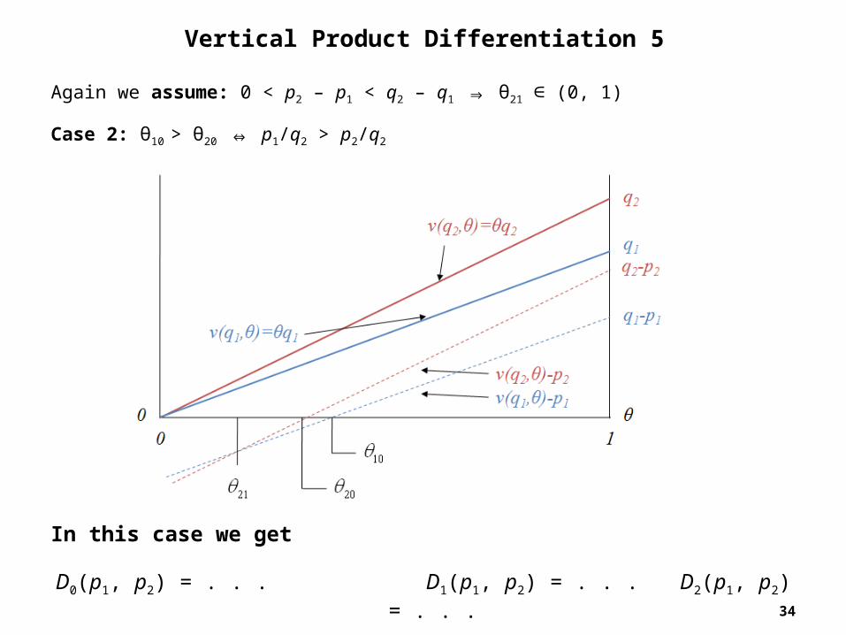
Vertical Product Differentiation 5
Again we assume: 0 < p2 – p1 < q2 – q1 ⇒ θ21 (0, 1) ∈
Case 2: θ10 > θ20 ⇔ p1/q2 > p2/q2
34
FIGURE HERE: 8
In this case we get
D0(p1, p2) = . . . D1(p1, p2) = . . . D2(p1, p2) = . . .

Horizontal Product Differentiation 1
Defining Features:
• consumers have different attitudes toward the characteristic q
• one consumer has a higher willingness to pay for qi than for qj, another a consumer
might still have a higher willingness to pay more for qj than for qi
Examples: taste of the ice-cream; color, design, or size of the T-shirt; location of the good;
An important subclass of this class of models is the class of models of spatial
differentiation.
In models of spatial differentiation
• q is the place of availability of the product (which is otherwise homogeneous)
• θ is consumer θ’s location
• preferences of consumers are different because the distance between own location and
the location of a particular product is different for different consumers and because
distance entails costs
Lecture 1: Roadmap, Contents, Basic Concepts 35

Horizontal Product Differentiation 2
A Simple Model of Spatial Differentiation (Hotelling 1929)
• goods are characterized by their location q in a city represented as lying on a line
segment of length 1: q ∈ [0, 1]
• consumers are characterized by their address θ on the same line segment
• consumers’ addresses are uniformly distributed on [0, 1]
• gross willingness to pay is r for each consumer
• consumption entails “travel cost” t/2 per unit of distance, where distance is 2|θ – q|
• the net willingness to pay of a consumer with address θ for a good located at q is
v(q,θ) = r - t|θ – q|
• the mass of consumers is normalized to 1
Note that there is also a non-spatial interpretation of this model, where
• q is a non-location related product characteristic
• θ is the ideal product characteristic from consumer θ‘s perspective
• consumer experiences a utility loss from consuming a product different from the
ideal one, and utility loss is proportional to the distance between θ and q
Lecture 1: Roadmap, Contents, Basic Concepts 36
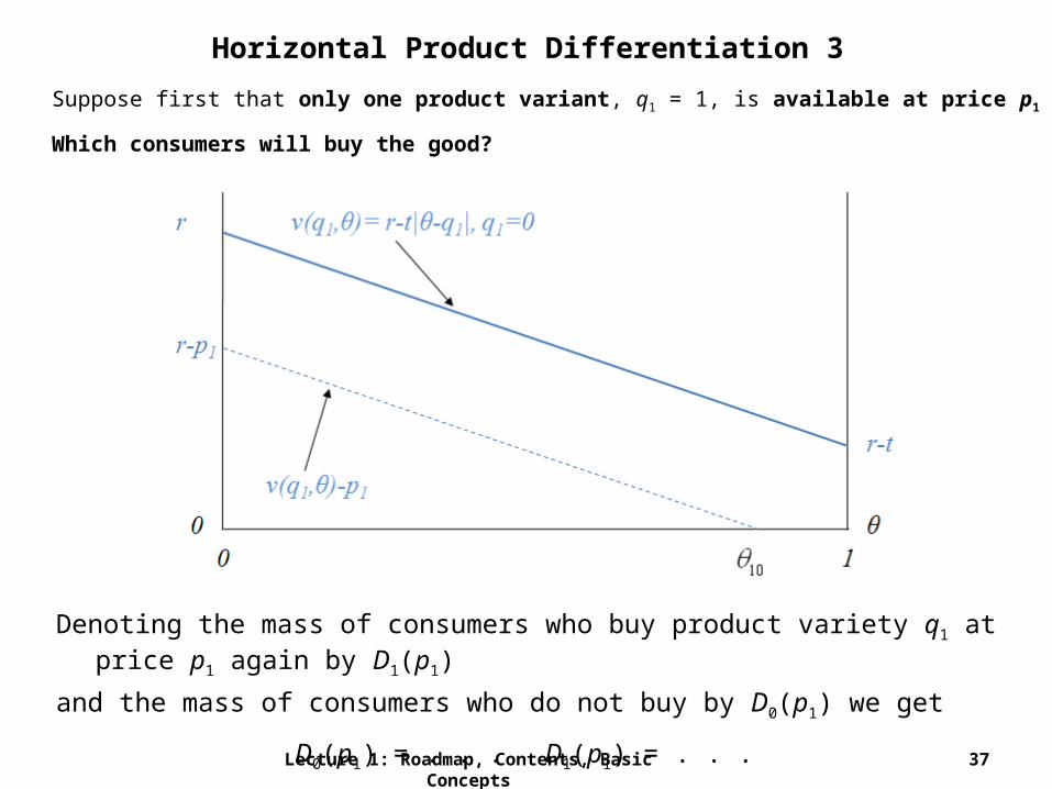
Horizontal Product Differentiation 3
Suppose first that only one product variant, q1 = 1, is available at price p1
Which consumers will buy the good?
Lecture 1: Roadmap, Contents, Basic Concepts 37
FIGURE HERE: 9
Denoting the mass of consumers who buy product variety q1 at price p1 again by D1(p1)
and the mass of consumers who do not buy by D0(p1) we get
D0(p1) = . . . D1(p1) = . . .
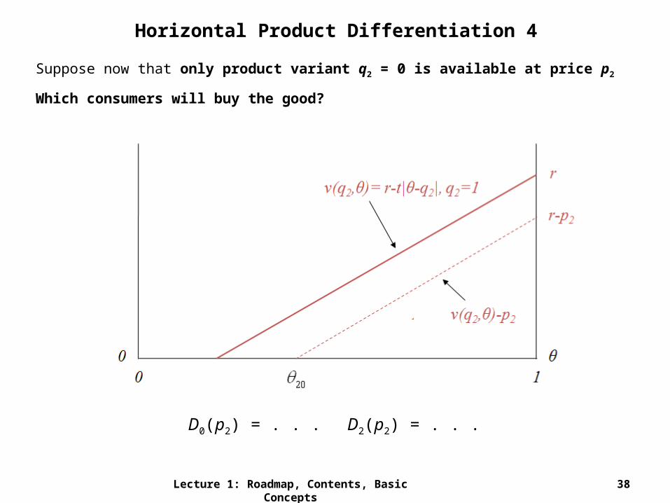
Horizontal Product Differentiation 4
Suppose now that only product variant q2 = 0 is available at price p2
Which consumers will buy the good?
Lecture 1: Roadmap, Contents, Basic Concepts 38
D0(p2) = . . . D2(p2) = . . .
FIGURE HERE: 10
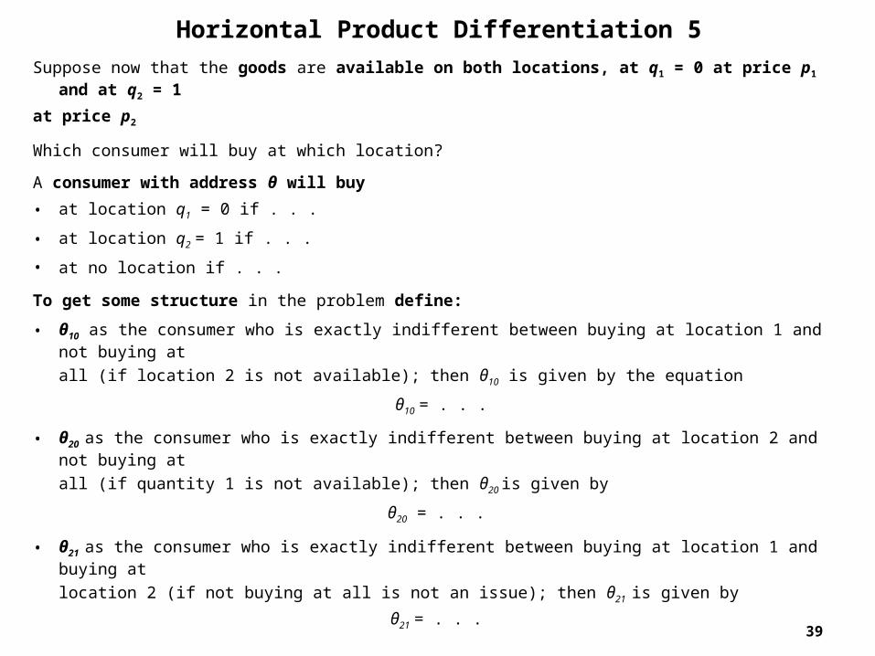
Horizontal Product Differentiation 5
Suppose now that the goods are available on both locations, at q1 = 0 at price p1 and at q2 = 1
at price p2
Which consumer will buy at which location?
A consumer with address θ will buy
• at location q1 = 0 if . . .
• at location q2 = 1 if . . .
• at no location if . . .
To get some structure in the problem define:
• θ10 as the consumer who is exactly indifferent between buying at location 1 and not buying at
all (if location 2 is not available); then θ10 is given by the equation
θ10 = . . .
• θ20 as the consumer who is exactly indifferent between buying at location 2 and not buying at
all (if quantity 1 is not available); then θ20 is given by
θ20 = . . .
• θ21 as the consumer who is exactly indifferent between buying at location 1 and buying at
location 2 (if not buying at all is not an issue); then θ21 is given by
θ21 = . . . 39
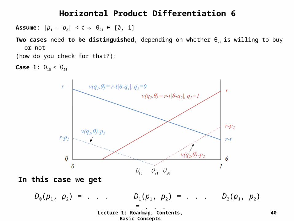
Horizontal Product Differentiation 6
Assume: |p1 – p2| < t ⇒ θ21 [0, 1] ∈
Two cases need to be distinguished, depending on whether θ21 is willing to buy or not
(how do you check for that?):
Case 1: θ10 < θ20
Lecture 1: Roadmap, Contents, Basic Concepts 40
FIGURE HERE: 11
In this case we get
D0(p1, p2) = . . . D1(p1, p2) = . . . D2(p1, p2) = . . .

Horizontal Product Differentiation 7
Again we assume: |p1 – p2| < t ⇒ θ21 [0, 1] ∈
Case 2: θ10 > θ20
Lecture 1: Roadmap, Contents, Basic Concepts 41
FIGURE HERE: 11
In this case we get
D0(p1, p2) = . . . D1(p1, p2) = . . . D2(p1, p2) = . . .

Horizontal Product Differentiation 8Up to now we have assumed
• prices are exogenously given
• product variety is exogenously given
• product characteristics are exogenously given
Later we want to endogenize each of these variables
• endogenizing prices is no problem in Hotelling
• endogenizing product variety might lead to problems because of asymmetries ⇨ Salop
• endogenizing p. characteristics might lead to problems as profits discontinuous in own price:
42
Effect of a small decrease in price (from p1 to p1’) in Hotelling
FIGURE HERE: 12 FIGURE HERE: 13

Horizontal Product Differentiation 9
Solution to the Discontinuity Problem:
D’Aspremont et al. (1979): linear city with v(q,θ) = r – t(q – θ)2
43
Solution to the Asymmetry Problem:
Salop (1979): circular city with v(q,θ) = r – t |q – θ|