Lecture 1: Mathematical roots - Harvard...
30
E-320: Teaching Math with a Historical Perspective O. Knill, 2010-2015 Lecture 1: Mathematical roots Similarly, as one has distinguished the canons of rhetorics: memory, invention, delivery, style, and arrangement, or combined the trivium: grammar, logic and rhetorics, with the quadrivium: arithmetic, geometry, music, and astronomy, to obtain the seven liberal arts and sciences, one has tried to organize all mathematical activities. Historically, one has dis- tinguished eight ancient roots of mathematics. Each of these 8 activities in turn suggest a key area in mathematics: counting and sorting arithmetic spacing and distancing geometry positioning and locating topology surveying and angulating trigonometry balancing and weighing statics moving and hitting dynamics guessing and judging probability collecting and ordering algorithms To morph these 8 roots to the 12 mathematical areas covered in this class, we complemented the ancient roots with calculus, numerics and computer science, merge trigonometry with geometry, separate arithmetic into number theory, algebra and arithmetic and turn statics into analysis. Lets call this modern adap- tation the 12 modern roots of Mathematics: counting and sorting arithmetic spacing and distancing geometry positioning and locating topology dividing and comparing number theory balancing and weighing analysis moving and hitting dynamics guessing and judging probability collecting and ordering algorithms slicing and stacking calculus operating and memorizing computer science optimizing and planning numerics manipulating and solving algebra While relating math- ematical areas with human activities is useful, it makes sense to select specific top- ics in each of this area. These 12 topics will be the 12 lectures of this course. Arithmetic numbers and number systems Geometry invariance, symmetries, measurement, maps Number theory Diophantine equations, factorizations Algebra algebraic and discrete structures Calculus limits, derivatives, integrals Set Theory set theory, foundations and formalisms Probability combinatorics, measure theory and statistics Topology polyhedra, topological spaces, manifolds Analysis extrema, estimates, variation, measure Numerics numerical schemes, codes, cryptology Dynamics differential equations, maps Algorithms computer science, artificial intelligence
Transcript of Lecture 1: Mathematical roots - Harvard...

E-320: Teaching Math with a Historical Perspective O. Knill, 2010-2015
Lecture 1: Mathematical roots
Similarly, as one has distinguished the canons of rhetorics: memory, invention, delivery, style,
and arrangement, or combined the trivium: grammar, logic and rhetorics, with the quadrivium:
arithmetic, geometry, music, and astronomy, to obtain the seven liberal arts and sciences, one
has tried to organize all mathematical activities.
Historically, one has dis-
tinguished eight ancient
roots of mathematics.
Each of these 8 activities in
turn suggest a key area in
mathematics:
counting and sorting arithmetic
spacing and distancing geometry
positioning and locating topology
surveying and angulating trigonometry
balancing and weighing statics
moving and hitting dynamics
guessing and judging probability
collecting and ordering algorithms
To morph these 8 roots to the 12 mathematical areas covered in this class, we complemented the
ancient roots with calculus, numerics and computer science, merge trigonometry with geometry,
separate arithmetic into number theory, algebra and arithmetic and turn statics into analysis.
Lets call this modern adap-
tation the
12 modern roots of
Mathematics:
counting and sorting arithmetic
spacing and distancing geometry
positioning and locating topology
dividing and comparing number theory
balancing and weighing analysis
moving and hitting dynamics
guessing and judging probability
collecting and ordering algorithms
slicing and stacking calculus
operating and memorizing computer science
optimizing and planning numerics
manipulating and solving algebra
While relating math-
ematical areas with
human activities is
useful, it makes sense
to select specific top-
ics in each of this area.
These 12 topics will be
the 12 lectures of this
course.
Arithmetic numbers and number systems
Geometry invariance, symmetries, measurement, maps
Number theory Diophantine equations, factorizations
Algebra algebraic and discrete structures
Calculus limits, derivatives, integrals
Set Theory set theory, foundations and formalisms
Probability combinatorics, measure theory and statistics
Topology polyhedra, topological spaces, manifolds
Analysis extrema, estimates, variation, measure
Numerics numerical schemes, codes, cryptology
Dynamics differential equations, maps
Algorithms computer science, artificial intelligence

Like any classification, this chosen division is rather arbitrary and a matter of personal preferences.
The 2010 AMS classification distinguishes 63 areas of mathematics. Many of the just defined
main areas are broken off into even finer pieces. Additionally, there are fields which relate with
other areas of science, like economics, biology or physics:
00 General01 History and biography03 Mathematical logic and foundations05 Combinatorics06 Lattices, ordered algebraic structures08 General algebraic systems11 Number theory12 Field theory and polynomials13 Commutative rings and algebras14 Algebraic geometry15 Linear/multi-linear algebra; matrix theory16 Associative rings and algebras17 Non-associative rings and algebras18 Category theory, homological algebra19 K-theory20 Group theory and generalizations
45 Integral equations46 Functional analysis47 Operator theory49 Calculus of variations, optimization51 Geometry52 Convex and discrete geometry53 Differential geometry54 General topology55 Algebraic topology57 Manifolds and cell complexes58 Global analysis, analysis on manifolds60 Probability theory and stochastic processes62 Statistics65 Numerical analysis68 Computer science70 Mechanics of particles and systems
22 Topological groups, Lie groups26 Real functions28 Measure and integration30 Functions of a complex variable31 Potential theory32 Several complex variables, analytic spaces33 Special functions34 Ordinary differential equations35 Partial differential equations37 Dynamical systems and ergodic theory39 Difference and functional equations40 Sequences, series, summability41 Approximations and expansions42 Fourier analysis43 Abstract harmonic analysis44 Integral transforms, operational calculus
74 Mechanics of deformable solids76 Fluid mechanics78 Optics, electromagnetic theory80 Classical thermodynamics, heat transfer81 Quantum theory82 Statistical mechanics, structure of matter83 Relativity and gravitational theory85 Astronomy and astrophysics86 Geophysics90 Operations research, math. programming91 Game theory, Economics Social and Behavioral Sciences92 Biology and other natural sciences93 Systems theory and control94 Information and communication, circuits97 Mathematics education
What are
fancy developments
in mathematics today? Michael
Atiyah identified in the year 2000
the following six hot spots:
local and global
low and high dimension
commutative and non-commutative
linear and nonlinear
geometry and algebra
physics and mathematics
Also this choice is of course highly personal. One can easily add 12 other polarizing quantities
which help to distinguish or parametrize different parts of mathematical areas, especially the
ambivalent pairs which produce a captivating gradient:
regularity and randomness
integrable and non-integrable
invariants and perturbations
experimental and deductive
polynomial and exponential
applied and abstract
discrete and continuous
existence and construction
finite dim and infinite dimensional
topological and differential geometric
practical and theoretical
axiomatic and case based
An other possibility to refine the fields of mathematics is to combine different of the 12 areas.
Examples are probabilistic number theory, algebraic geometry, numerical analysis, ge-
ometric number theory, numerical algebra, algebraic topology, geometric probability,
algebraic number theory, dynamical probability = stochastic processes. Almost every
pair is an actual field. Finally, lets give a short answer to the question: What is Mathematics?
Mathematics is the science of structure.
The goal is to illustrate some of these structures from a historical point of view.

E-320: Teaching Math with a Historical Perspective Oliver Knill, 2010-2015
Lecture 2: Arithmetic
The oldest mathematical discipline is Arithmetic, the theory of constructing and manipulatingnumbers. The earliest steps were done by Babylonian, Egyptian, Chinese, Indian and Greek
thinkers. Building up the number system starts with the natural numbers 1, 2, 3, 4... where onecan add and multiply. While addition is natural: when adding 3 sticks to 5 sticks to get 8 sticks,the multiplicative operation ∗ is more subtle: 3 ∗ 4 can be read that we take 3 copies of 4 and get4 + 4+ 4 = 12. And 4 ∗ 3 means we take 4 copies of 3 to get 3 + 3+ 3+ 3 = 12. The first numbercounts the number of operations while the second counts objects. To motivate 3 ∗ 4 = 4 ∗ 3,spacial insight can help: we can arrange the 12 objects in a rectangle. Realizing an addition andmultiplication structure on the natural numbers is a great moment in mathematics. It leadsnaturally to more general numbers. There are two major motivations to to build new numbers:
1. invert operations and still get results. 2. solve equations.
For 1. to find an inverse of 3 means finding a number such that x + 3 = 0 we need x = −3, anegative number, to find a number such that x3 = 1, we need x = 1/3, a rational number. For 2.,in order to solve x+3 = 1 one needs integers, to solve 3x = 4 one needs fractions, to solve x2 = 2one needs real numbers, to solve x2 = −2 one needs complex numbers.
Numbers Operation to complete Examples of equations to solveNatural numbers addition and multiplication 5 + x = 9Positive fractions addition and division 5x = 8Integers also subtraction 5 + x = 3Rational numbers also division 3x = 5Algebraic numbers taking positive roots x2 = 2 , 2x+ x2 − x3 = 2Real numbers taking limits x = 1− 1/3 + 1/5−+...,cos(x) = xComplex numbers take any roots x2 = −2Surreal numbers transfinite limits x2 = ω, 1/x = ωSurreal complex any operation x2 + 1 = −ω
The development and history of arithmetic can be summarized as follows: humans started withnatural numbers, dealt with positive fractions, reluctantly introduced negative numbers and zero toget integers, struggled to ”realize” real numbers, were scared to introduce complex numbers, hardlyaccepted surreal numbers and most do not even know about surcomplex numbers. Ironically, assimple but impossibly difficult questions in number theory show, the modern point of view is theopposite to Kronecker’s ”God made the integers; all else is the work of man”:
The surreal complex numbers are the most natural numbers;The natural numbers are the most complex, surreal numbers.
Natural numbers. Counting can be realized by sticks, bones, quipu knots, pebbles or wampumknots. The tally stick concept is still used when playing card games: where bundles of fives areformed, maybe by crossing 4 ”sticks” with a fifth. An old stone age tally stick, the wolf radius
bone contains 55 notches, with 5 groups of 5. It is probably more than 30’000 years old. An otherfamous paleolithic tally stick is the Ishango bone, the fibula of a baboon. It could be 20’000 -30’000 years old. Others date it to 9000-6500 BC. Earlier counting could have been done by assem-bling pebbles, tying knots in a string, making scratches in dirt or bark but no such traces have

survived the thousands of years. The Roman system improved the tally stick concept by intro-ducing new symbols for larger numbers like V = 5, X = 10, L = 40, C = 100, D = 500,M = 1000.in order to avoid bundling too many single sticks. The system is unfit for computations as sim-ple calculations V III + V II = XV show. Clay tablets, some as early as 2000 BC and othersfrom 600 - 300 BC are known. They feature Akkadian arithmetic using the base 60. Thehexadecimal system with base 60 is convenient becuase of many factors. It survived: we use 60minutes per hour. The Egyptians used the base 10. The most important source on Egyptianmathematics is the Rhind Papyrus of 1650 BC. Hieratic numerals were used to write on pa-pyrus from 2500 BC on. Egyptian numerals are hieroglyphics. They were found in carvings ontombs and monuments and are 5000 years old. The modern way to write numbers like 2015 is theHindu-Arab system which diffused to the West only during the late Middle ages. It replacedthe more primitive Roman system. Greek arithmetic used a primitive number system with noplace values: 9 Greek letters for 1, 2, . . . 9, nine for 10, 20, . . . , 90 and nine for 100, 200, . . . , 900.
Integers. Indian Mathematics morphed the place-value system into a modern method ofwriting numbers. Hindu astronomers used words to represent digits, but the numbers would bewritten in the opposite order. Sometimes after 500, the Hindus changed to a digital notationwhich included the symbol 0. Negative numbers were introduced around 100 BC in the Chinese
text ”Nine Chapters on the Mathematica art”. Also the Bakshali manuscript, written around300 AD subtracts numbers carried out additions with negative numbers, where + was used toindicate a negative sign. In Europe, negative numbers were avoided until the 15’th century.
Fractions: Babylonians could handle fractions. The Egyptians also used fractions, but wroteevery fraction a as a sum of fractions with unit numerator and distinct denominators, like4/5 = 1/2 + 1/4 + 1/20 or 5/6 = 1/2 + 1/3. Maybe because of such cumbersome computa-tion techniques, Egyptian mathematics failed to progress beyond a primitive stage. The moderndecimal fractions used nowadays for numerical calculations were adopted only in 1595 in Europe.
Real numbers: The Greeks who noticed first that the diagonal of the square is not a rationalnumber. It produced a crisis. Only much later, it became clear that ”most” numbers are notrational. Georg Cantor realized first that the cardinality of all real numbers is much larger thanthe cardinality of the integers: while one can count all rational numbers but not enumerate allreal numbers. One consequence is that most real numbers are transcendental: they do not occuras solutions of polynomial equations with integer coefficients. The number π is an example. Theconcept of real numbers is related to th concept of limit. Sums like 1+1/4+1/9+1/16+1/25+...approach real numbers which are not rational any more.
Complex numbers: Some polynomials have no real root. To solve x2 = −1 for example, we neednew numbers. One idea is to use pairs of numbers (a, b) where (a, 0) = a are the usual numbers andextend addition and multiplication (a, b)+(c, d) = (a+c, b+d) and (a, b)·(c, d) = (ac−bd, ad+bc).With this multiplication, the number (0, 1) has the property that (0, 1) · (0, 1) = (−1, 0) = −1. Itis more convenient to write a+ ib where i = (0, 1) satisfies i2 = −1. One can now use the commonrules of addition and multiplication.
Surreal numbers: Similarly as real numbers fill in the gaps between the integers, the surrealnumbers fill in the gaps between Cantors ordinal numbers. They are written as (a, b, c, ...|d, e, f, ...)meaning that the ”simplest” number is larger than a, b, c... and smaller than d, e, f, ... We have(|) = 0, (0|) = 1, (1|) = 2 and (0|1) = 1/2 or (|0) = −1. Surreals contain already transfinite num-bers like (0, 1, 2, 3...|) or infinitesimal numbers like (0|1/2, 1/3, 1/4, 1/5, ...). They were introducedin the 1970’ies by John Conway. The late appearance confirms the pedagogical principle: late
human discovery manifests in increased difficulty to teach it.

E-320: Teaching Math with a Historical Perspective Oliver Knill, 2010-2015
Lecture 3: Geometry
Geometry is the science of shape, size and symmetry. While arithmetic dealt with numericalstructures, geometry deals with metric structures. Geometry is one of the oldest mathemati-cal disciplines and early geometry has relations with arithmetics: we have seen that that theimplementation of a commutative multiplication on the natural numbers is rooted from an inter-pretation of n×m as an area of a shape that is invariant under rotational symmetry. Numbersystems built upon the natural numbers inherit this. Identities like the Pythagorean triples
32+42 = 52 were interpreted geometrically. The right angle is the most ”symmetric” angle apartfrom 0. Symmetry manifests itself in quantities which are invariant. Invariants are one the mostcentral aspects of geometry. Felix Klein’s Erlanger program uses symmetry to classify geome-tries depending on how large the symmetries of the shapes are. In this lecture, we look at a fewresults which can all be stated in terms of invariants. In the presentation as well as the worksheetpart of this lecture, we will work us through smaller miracles like special points in triangles aswell as a couple of gems: Pythagoras, Thales,Hippocrates, Feuerbach, Pappus, Morley,Butterfly which illustrate the importance of symmetry.
Much of geometry is based on our ability to measure length, the distance between two points.A modern way to measure distance is to determine how long light needs to get from one pointto the other. This geodesic distance generalizes to curved spaces like the sphere and is also apractical way to measure distances, for example with lasers. It bypasses the problem to determinefirst the underlying nature of the space in which we do geometry. Having a distance d(A,B)between any two points A,B, we can look at the next more complicated object, which is a setA,B,C of 3 points, a triangle. Given an arbitrary triangle ABC, are there relations between the3 possible distances a = d(B,C), b = d(A,C), c = d(A,B)? If we fix the scale by c = 1, thena + b ≥ 1, a + 1 ≥ b, b + 1 ≥ a. For any pair of (a, b) in this region, there is a triangle. Afteran identification, we get an abstract space, which represent all triangles uniquely up to similarity.Mathematicians call this an example of a moduli space.
A sphere Sr(x) is the set of points which have distance r from a given point x. In the plane, thesphere is called a circle. A natural problem is to find the circumference L = 2π of a unit circle,or the area A = π of a unit disc, the area F = 4π of a unit sphere and the volume V = 4 = π/3 ofa unit sphere. Measuring the length of segments on the circle leads to new concepts like angle orcurvature. Because the circumference of the unit circle in the plane is L = 2π, angle questionsare tied to the number π, which Archimedes already approximated by fractions.
Also volumes were among the first quantities, Mathematicians wanted to measure and com-pute. A problem on Moscow papyrus dating back to 1850 BC explains the general formulah(a2+ab+b2)/3 for a truncated pyramid with base length a, roof length b and height h. Archimedesachieved to compute the volume of the sphere: place a cone inside a cylinder. The complementof the cone inside the cylinder has on each height h the area π−πh2. The half sphere cut at heighth is a disc of radius (1 − h2) which has area π(1 − h2) too. Since the slices at each height havethe same area, the volume must be the same. The complement of the cone inside the cylinder hasvolume π − π/3 = 2π/3, half the volume of the sphere.
The first geometric playground was planimetry, the geometry in the flat two dimensional space.Highlights are Pythagoras theorem, Thales theorem, Hippocrates theorem, and Pappus

theorem. Discoveries in planimetry have been made later on: an example is the Feuerbachtheorem from the 19th century or the Sadov theorem for quadrilaterals. Greek Mathematics isclosely related to history. It starts with Thales goes over Euclid’s era at 300 BC, and endswith the threefold destruction of Alexandria 47 BC by the Romans, 392 by the Christians and640 by the Muslims. Geometry was also a place, where the axiomatic method was broughtto mathematics: theorems are proved from a few statements which are called axioms like the 5axioms of Euclid:
1. Any two distinct points A,B determines a line through A and B.2. A line segment [A,B] can be extended to a straight line containing the segment.3. A line segment [A,B] determines a circle containing B and center A.4. All right angles are congruent.5. If lines L,M intersect with a third so that inner angles add up to < π, then L,M intersect.
Euclid wondered whether the fifth postulate can be derived from the first four and called theo-rems derived from the first four the ”absolute geometry”. Only much later, with Karl-Friedrich
Gauss and Janos Bolyai and Nicolai Lobachevsky in the 19’th century in hyperbolic space
the 5’th axiom does not hold. Indeed, geometry can be generalized to non-flat, or even much moreabstract situations. Basic examples are geometry on a sphere leading to spherical geometry orgeometry on the Poincare disc, a hyperbolic space. Both of these geometries are non-Euclidean.Riemannian geometry, which is essential for general relativity theory generalizes both con-cepts to a great extent. An example is the geometry on an arbitrary surface. Curvatures of suchspaces can be computed by measuring length alone, which is how long light needs to go from onepoint to the next.
An important moment in mathematics was the merge of geometry with algebra: this giantstep is often attributed to Rene Descartes. Together with algebra, the subject leads to algebraicgeometry which can be tackled with computers: here are some examples of geometries which aredetermined from the amount of symmetry which is allowed:
Euclidean geometry Properties invariant under a group of rotations and translationsAffine geometry Properties invariant under a group of affine transformationsProjective geometry Properties invariant under a group of projective transformationsSpherical geometry Properties invariant under a group of rotationsConformal geometry Properties invariant under angle preserving transformationsHyperbolic geometry Properties invariant under a group of Mobius transformations
Here are four pictures about the 4 special points in a triangle and with which we will begin. Wewill see why in each of these cases, the 3 lines intersect in a common point. It is a manifestationof a symmetry present on the space of all triangles. size of the distance of intersection points isconstant 0 if we move on the space of all triangular shapes. It’s Geometry!

E-320: Teaching Math with a Historical Perspective Oliver Knill, 2010-2015
Lecture 4: Number Theory
Number theory studies the structure of integers like prime numbers and solutions to Diophantineequations. Gauss called it the ”Queen of Mathematics”. Here are a few theorems and open prob-lems.An integer larger than 1 which is divisible by 1 and itself only is called a prime number.The number 257885161 − 1 is the largest known prime number. It has 17425170 digits. Euclid
proved that there are infinitely many primes: [Proof. Assume there are only finitely many primesp1 < p2 < . . . < pn. Then n = p1p2 · · ·pn + 1 is not divisible by any p1, . . . , pn. Therefore, it is aprime or divisible by a prime larger than pn.] Primes become more sparse as larger as they get. Animportant result is the prime number theorem which states that the n’th prime number hasapproximately the size n log(n). For example the n = 1012’th prime is p(n) = 29996224275833 andn log(n) = 27631021115928.545... and p(n)/(n log(n)) = 1.0856... Many questions about primenumbers are unsettled: Here are four problems: the third uses the notation (∆a)n = |an+1−an| toget the absolute difference. For example: ∆2(1, 4, 9, 16, 25...) = ∆(3, 5, 7, 9, 11, ...) = (2, 2, 2, 2, ...).Progress on prime gaps has been done recently: a paper which just appears showed pn+1 − pn issmaller than 100’000’000 eventually (Yitang Zhang April 2013) pn+1−pn is smaller than 600 even-tually (Maynard) . The largest known gap is 1476 which occurs after p = 1425172824437699411.
Twin prime there are infinitely many primes p such that p+ 2 is prime.Goldbach every even integer n > 2 is a sum of two primes.Gilbreath If pn enumerates the primes, then (∆kp)1 = 1 for all k > 0.Andrica The prime gap estimate
√pn+1 −
√pn < 1 holds for all n.
If the sum of the proper divisors of a n is equal to n, then n is called a perfect number.For example, 6 is perfect as its proper divisors 1, 2, 3 sum up to 6. All currently known per-fect numbers are even. The question whether odd perfect numbers exist is probably the oldestopen problem in mathematics and not settled. Perfect numbers were familiar to Pythagorasand his followers already. Calendar coincidences like that we have 6 work days and the moonneeds ”perfect” 28 days to circle the earth could have helped to promote the ”mystery” of per-fect number. Euclid of Alexandria (300-275 BC) was the first to realize that if 2p − 1 isprime then k = 2p−1(2p − 1) is a perfect number: [Proof: let σ(n) be the sum of all factors ofn, including n. Now σ(2n − 1)2n−1) = σ(2n − 1)σ(2n−1) = 2n(2n − 1) = 2 · 2n(2n − 1) showsσ(k) = 2k and verifies that k is perfect.] Around 100 AD, Nicomachus of Gerasa (60-120)classified in his work ”Introduction to Arithmetic” numbers on the concept of perfect numbersand lists four perfect numbers. Only much later it became clear that Euclid got all the evenperfect numbers: Euler showed that all even perfect numbers are of the form (2n − 1)2n−1, where2n − 1 is prime. The factor 2n − 1 is called a Mersenne prime. [Proof: Assume N = 2kmis perfect where m is odd and k > 0. Then 2k+1m = 2N = σ(N) = (2k+1 − 1)σ(m). Thisgives σ(m) = 2k+1m/(2k+1 − 1) = m(1 + 1/(2k+1 − 1)) = m +m/(2k+1 − 1). Because σ(m) andm are integers, also m/(2k+1 − 1) is an integer. It must also be a factor of m. The only waythat σ(m) can be the sum of only two of its factors is that m is prime and so 2k+1 − 1 = m.]The first 39 known Mersenne primes are of the form 2n − 1 with n = 2, 3, 5, 7, 13, 17, 19,31, 61, 89, 107, 127, 521, 607, 1279, 2203, 2281, 3217, 4253, 4423, 9689, 9941, 11213, 19937,21701, 23209, 44497, 86243, 110503, 132049, 216091, 756839, 859433, 1257787, 1398269, 2976221,3021377, 6972593, 13466917. There are 8 more known from which one does not know the rankof the corresponding Mersenne prime: n = 20996011, 24036583, 25964951, 30402457, 32582657,
37156667, 42643801,43112609,57885161. The last was found in January 2013 only. It is unknownwhether there are infinitely many.
A polynomial equations for which all coefficients and variables are integers is called aDiophantine
equation. The first Diophantine equation studied already by Babilonians is x2 + y2 = z2. Asolution (x, y, z) of this equation in positive integers is called a Pythagorean triple. For example,(3, 4, 5) is a Pythagorean triple. Since 1600 BC, it is known that all solutions to this equationare of the form (x, y, z) = (2st, s2 − t2, s2 + t2) or (x, y, z) = (s2 − t2, 2st, s2 + t2), where s, t aredifferent integers. [Proof. Either x or y has to be even because if both are odd, then the sumx2 + y2 is even but not divisible by 4 but the right hand side is either odd or divisible by 4. Movethe even one, say x2 to the left and write x2 = z2 − y2 = (z − y)(z + y), then the right hand sidecontains a factor 4 and is of the form 4s2t2. Therefore 2s2 = z − y, 2t2 = z + y. Solving for z, ygives z = s2 + t2, y = s2 − t2, x = 2st.]Analyzing Diophantine equations can be difficult. Only 10 years ago, one has established that theFermat equation xn + yn = zn has no solutions with xyz 6= 0 if n > 2. Here are some open
problems for Diophantine equations. Are there nontrivial solutions to the following Diophantineequations?
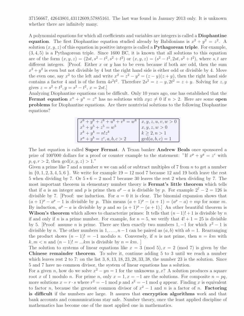
x6 + y6 + z6 + u6 + v6 = w6 x, y, z, u, v, w > 0x5 + y5 + z5 = w5 x, y, z, w > 0xk + yk = n!zk k ≥ 2, n > 1xa + yb = zc, a, b, c > 2 gcd(a, b, c) = 1
The last equation is called Super Fermat. A Texan banker Andrew Beals once sponsored aprize of 100′000 dollars for a proof or counter example to the statement: ”If xp + yq = zr withp, q, r > 2, then gcd(x, y, z) > 1.”Given a prime like 7 and a number n we can add or subtract multiples of 7 from n to get a numberin 0, 1, 2, 3, 4, 5, 6 . We write for example 19 = 12 mod 7 because 12 and 19 both leave the rest5 when dividing by 7. Or 5 ∗ 6 = 2 mod 7 because 30 leaves the rest 2 when dividing by 7. Themost important theorem in elementary number theory is Fermat’s little theorem which tellsthat if a is an integer and p is prime then ap − a is divisible by p. For example 27 − 2 = 126 isdivisible by 7. [Proof: use induction. For a = 0 it is clear. The binomial expansion shows that(a + 1)p − ap − 1 is divisible by p. This means (a + 1)p − (a + 1) = (ap − a) + mp for some m.By induction, ap − a is divisible by p and so (a + 1)p − (a + 1).] An other beautiful theorem isWilson’s theorem which allows to characterize primes: It tells that (n− 1)!+ 1 is divisible by nif and only if n is a prime number. For example, for n = 5, we verify that 4! + 1 = 25 is divisibleby 5. [Proof: assume n is prime. There are then exactly two numbers 1,−1 for which x2 − 1 isdivisible by n. The other numbers in 1, . . . , n−1 can be paired as (a, b) with ab = 1. Rearrangingthe product shows (n − 1)! = −1 modulo n. Conversely, if n is not prime, then n = km withk,m < n and (n− 1)! = ...km is divisible by n = km. ]The solution to systems of linear equations like x = 3 (mod 5), x = 2 (mod 7) is given by theChinese remainder theorem. To solve it, continue adding 5 to 3 until we reach a numberwhich leaves rest 2 to 7: on the list 3, 8, 13, 18, 23, 28, 33, 38, the number 23 is the solution. Since5 and 7 have no common divisor, the system of linear equations has a solution.For a given n, how do we solve x2 − yn = 1 for the unknowns y, x? A solution produces a squareroot x of 1 modulo n. For prime n, only x = 1, x = −1 are the solutions. For composite n = pq,more solutions x = r · s where r2 = −1 mod p and s2 = −1 mod q appear. Finding x is equivalentto factor n, because the greatest common divisor of x2 − 1 and n is a factor of n. Factoring
is difficult if the numbers are large. It assures that encryption algorithms work and thatbank accounts and communications stay safe. Number theory, once the least applied discipline ofmathematics has become one of the most applied one in mathematics.

E-320: Teaching Math with a Historical Perspective Oliver Knill, 2012-2015
Lecture 4: Number Theory
Twin prime conjecture
There are infinitely many prime twins p, p+ 2.
The first twin prime is (3, 5). The largest knownprime twins (p, p + 2) have been found in 2011. It is3756801695685 · 2666669 ± 1. There are analogue prob-lems for cousin primes p, p+4, sexy primes p, p+6 orGermaine primes, where p, 2p+1 are prime. Progress:we know that prime gaps of order 600 or smaller appearinfinitely often. (Work of Zhang,Maynard,Tao)
Goldbach conjecture
Every even integer n > 2 is a sum of two primes.
The Goldbach conjecture has been verified numericallyuntil 4·1018. It is known that every sufficiently large oddnumber is the sum of 3 primes. One believes this ”weakGoldbach conjecture” for 3 primes is true for every oddinteger larger than 7.
Andrica conjecture
The prime gap estimate√pn+1 −
√pn < 1 holds.
For example√p1000−
√p999 =
√7919−
√7907 = 0.067....
An other prime gap estimate conjectures is Polignac’sconjecture claiming that there are infinitely manyprime gaps for every even number n. It is stronger thanthe twin prime conjecture. It includes for example theclaim that there are infinitely many cousin primes orsexy primes. Legendre’s conjecture claims that thereexists a prime between any two perfect squares. Between16 = 42 and 25 = 52, there is the prime 23 for example.

Odd perfect numbers
Probably the oldest open problem in mathematics is thequestion
There is an odd perfect number.
A perfect number is equal to the sum of all its properpositive divisors. Like 6 = 1 + 2 + 3. The search forperfect numbers is related to the search of large primenumbers. The largest prime number known today isp = 243112609 − 1. It is called a Mersenne prime. Everyeven perfect number is of the form 2n−1(2n − 1) where2n − 1 is prime.
Diophantine equations
Many problems about Diophantine equations, equationswith integer solutions are unsettled. Here is an example:
Solve x5 + y5 + z5 = w5 for x, y, z, w ∈ N .
Also x5 + y5 = u5 + v5 has no nontrivial solutions yet.Probabilistic considerations suggest that there are nosolutions. The analogue equation x4 + y4 + z4 = w4
had been settled by Noam Elkies in 1988 who found theidentity 26824404+153656394+187967604 = 206156734.
ABC Conjecture
The abc conjecture is:
If a+ b = c, then c ≤ (∏
p|abc p)2.
For example, for 10+22 = 32, the prime factors of abc =7040 are 2, 5, 11 and indeed 32 ≤ (2 ∗ 5 ∗ 11)2 = 12100.The abc-conjecture is open but implies Fermat’s theo-rem for n ≥ 6: assume xn+yn = zn with coprime x, y, z.Take a = xn, b = yn, c = zn. The abc-conjecture giveszn ≤ (
∏p|abc p) ≤ (abc)2 < z6 establishing Fermat for
n ≥ 6. The cases n = 3, 4, 5 to Fermat have been knownfor a long time. In August 2012, there were rumors ofan attack by Shinichi Mochizuki. During 2013 variousmathematicians have tried to understand and verify thetheory.

E-320: Teaching Math with a Historical Perspective Oliver Knill, 2010-2015
Lecture 5: Algebra
Algebra studies algebraic structures like ”groups” and ”rings”. The theory allows to solvepolynomial equations, characterize objects by its symmetries and is the heart and soul of manypuzzles. Lagrange claimsDiophantus to be the inventor of Algebra, others argue that the subjectstarted with solutions of quadratic equation by Mohammed ben Musa Al-Khwarizmi inthe book Al-jabr w’al muqabala of 830 AD. Solutions to equation like x2 + 10x = 39 are solvedthere by completing the squares: add 25 on both sides go get x2 + 10x + 25 = 64 and so(x+ 5) = 8 so that x = 3.The use of variables introduced in school in elementary algebra were introduced later. Ancienttexts only dealt with particular examples and calculations were done with concrete numbers in therealm of arithmetic. Francois Viete (1540-1603) used first letters like A,B,C,X for variables.
The search for formulas for polynomial equations of degree 3 and 4 lasted 700 years. In the16’th century, the cubic equation and quartic equations were solved. Niccolo Tartaglia andGerolamo Cardano reduced the cubic to the quadratic: [first remove the quadratic part withX = x−a/3 so that X3+aX2+bX+c becomes the depressed cubic x3+px+q. Now substitutex = u− p/(3u) to get a quadratic equation (u6 + qu3
− p3/27)/u3 = 0 for u3.] Lodovico Ferrari
shows that the quartic equation can be reduced to the cubic. For the quintic however no formulascould be found. It was Paolo Ruffini, Niels Abel and Evariste Galois who independentlyrealized that there are no formulas in terms of roots which allow to ”solve” equations p(x) = 0 forpolynomials p of degree larger than 4. This was an amazing achievement and the birth of ”grouptheory”.
Two important algebraic structures are groups and rings.
In a group G one has an operation ∗, an inverse a−1 and a one-element 1 such that a ∗ (b ∗ c) =(a ∗ b) ∗ c, a ∗ 1 = 1 ∗ a = a, a ∗ a−1 = a−1
∗ a = 1. For example, the set Q∗ of nonzero fractionsp/q with multiplication operation ∗ and inverse 1/a form a group. The integers with addition andinverse a−1 = −a and ”1”-element 0 form a group too. A ring R has two compositions + and ∗,where the plus operation is a group satisfying a + b = b+ a in which the one element is called 0.The multiplication operation ∗ has all group properties on R∗ except the existence of an inverse.The two operations + and ∗ are glued together by the distributive law a ∗ (b+ c) = a ∗ b+ a ∗ c.An example of a ring are the integers or the rational numbers or the real numbers. Thelater two are actually fields, rings for which the multiplication on nonzero elements is a grouptoo. The ring of integers are no field because an integer like 5 has no multiplicative inverse. Thering of rational numbers however form a field.
Why is the theory of groups and rings not part of arithmetic? First of all, a crucial ingredientof algebra is the appearance of variables and computations with these algebras without usingconcrete numbers. Second, the algebraic structures are not restricted to ”numbers”. Groups andrings are general structures and extend for example to objects like the set of all possible sym-metries of a geometric object. The set of all similarity operations on the plane for exampleform a group. An important example of a ring is the polynomial ring of all polynomials. Givenany ring R and a variable x, the set R[x] consists of all polynomials with coefficients in R. Theaddition and multiplication is done like in (x2 + 3x+ 1) + (x− 7) = x2 + 4x− 7. The problem to

for example can be written as (x+1)(x−2) have a number theoretical flavor. Because symmetriesof some structure form a group, we also have intimate connections with geometry. But this isnot the only connection with geometry. Geometry also enters through the polynomial rings withseveral variables. Solutions to f(x, y) = 0 leads to geometric objects with shape and symmetrywhich sometimes even have their own algebraic structure. They are called varieties, a centralobject in algebraic geometry.
Arithmetic introduces addition and multiplication of numbers. Both form a group. The operationscan be written additively or multiplicatively. Lets look at this a bit closer:For integers, fractions and reals and the addition +, the 1 element 0 and inverse −g, we have agroup. Many groups are written multiplicatively where the 1 element is 1. In the case of fractionsor reals, 0 is not part of the multiplicative group because it is not possible to divide by 0. Thenonzero fractions or the nonzero reals form a group. In all these examples the groups satisfy thecommutative law g ∗ h = h ∗ g.Here is a group which is not commutative: let G be the set of all rotations in space, whichleave the unit cube invariant. There are 3*3=9 rotations around each major coordinate axes,then 6 rotations around axes connecting midpoints of opposite edges, then 2*4 rotations arounddiagonals. Together with the identity rotation e, these are 24 rotations. The group operation isthe composition of these transformations.An other example of a group is S4, the set of all permutations of four numbers (1, 2, 3, 4). Ifg : (1, 2, 3, 4) → (2, 3, 4, 1) is a permutation and h : (1, 2, 3, 4) → (3, 1, 2, 4) is an other permutation,then we can combine the two and define h ∗ g as the permutation which does first g and then h.We end up with the permutation (1, 2, 3, 4) → (1, 2, 4, 3). The rotational symmetry group of thecube happens to be the same than the group S4. To see this ”isomorphism”, label the 4 spacediagonals in the cube by 1, 2, 3, 4. Given a rotation, we can look at the induced permutation ofthe diagonals and every rotation corresponds to exactly one permutation. The symmetry groupcan be introduced for any geometric object. For shapes like the triangle, the cube, the octahedronor tilings in the plane.
Symmetry groups describe geometric shapes by algebra.
Many puzzles are groups. A popular puzzle, the 15-puzzle was invented in 1874 by Noyes
Palmer Chapman in the state of New York. If the hole is given the number 0, then the taskof the puzzle is to order a given random start permutation of the 16 pieces. To do so, the user isallowed to transposes 0 with a neighboring piece. Since every step changes the signature s of thepermutation and changes the taxi-metric distance d of 0 to the end position by 1, only situationswith even s + d can be reached. It was Sam Loyd who suggested to start with an impossiblesolution and as an evil plot to offer 1000 dollars for a solution. The 15 puzzle group has 16!/2elements and the ”god number” is between 152 and 208. The Rubik cube is an other famouspuzzle, which is a group. Exactly 100 years after the invention of the 15 puzzle, the Rubik puzzlewas introduced in 1974. Its still popular and the world record is to have it solved in 5.55 seconds.Cubes 2x2x2 to 7x7x7 have been solved in a total time of 6 minutes. For the 3x3x3 cube, the godnumber is now known to be 20: one can always solve it in 20 or less moves.
Many puzzles are groups.
A small rubik type game is the ”floppy”, which is a third of the rubik and which has only 192elements. An other example is the Meffert’s great challenge. Probably the simplest exampleof a Rubik type puzzle is the pyramorphix. It is a puzzle based on the tetrahedron. Its grouphas only 24 elements. It is the group of all possible permutations of the 4 elements. It is thesame group as the group of all reflection and rotation symmetries of the cube in three dimensionsand also is relevant when understanding the solutions to the quartic equation discussed at the
E-320: Teaching Math with a Historical Perspective Oliver Knill, 2010-2015
Lecture 6: Calculus
Calculus formalizes the process of taking differences and taking sums. Differences measurechange, sums explore how things accumulate. The process of taking differences has a limitcalled derivative. The process of taking sums will lead to the integral. These two processes arerelated in an intimate way. In this lecture, we look at these two processes in the simplest possiblesetup, where functions are evaluated on integers and where we do not take any limits.Several dozen thousand years ago, numbers were represented by units like
1, 1, 1, 1, 1, 1, . . .
for example carved in the Ishango bone. It took thousands of years until numbers were representedwith symbols like
0, 1, 2, 3, 4, . . . .
Using the modern concept of function, we can say f(0) = 0, f(1) = 1, f(2) = 2, f(3) = 3 andmean that the function f assigns to an input like 1001 an output like f(1001) = 1001. Lets callDf(n) = f(n + 1)− f(n) the difference between two function values. We see that the functionf satisfies Df(n) = 1 for all n. We can also formalize the summation process. If g(n) = 1 is thefunction which is constant 1, then Sg(n) = g(0)+ g(1)+ . . .+ g(n− 1) = 1+ 1+ · · ·+1 = n. Wesee that Df = g and Sg = f . Lets start with f(n) = n and apply summation on that function:
Sf(n) = f(0) + f(1) + f(2) + · · ·+ f(n− 1) .
In our example, we get the values:
0, 1, 3, 6, 10, 15, 21, . . . .
The new function g = Sf satisfies g(1) = 1, g(2) = 3, g(2) = 6, etc. These numbers are calledtriangular numbers. From g we can get back f by taking difference:
Dg(n) = g(n+ 1)− g(n) = f(n) .
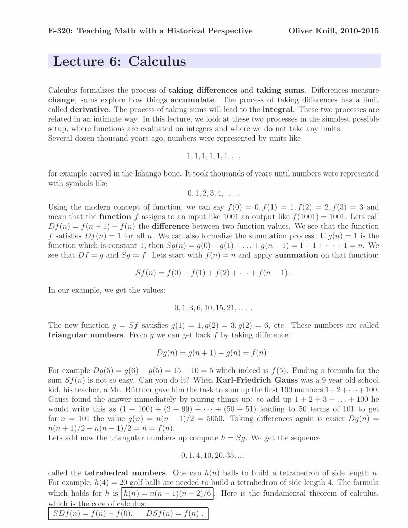
For example Dg(5) = g(6)− g(5) = 15 − 10 = 5 which indeed is f(5). Finding a formula for thesum Sf(n) is not so easy. Can you do it? When Karl-Friedrich Gauss was a 9 year old schoolkid, his teacher, a Mr. Buttner gave him the task to sum up the first 100 numbers 1+2+ · · ·+100.Gauss found the answer immediately by pairing things up: to add up 1 + 2 + 3 + . . . + 100 hewould write this as (1 + 100) + (2 + 99) + · · · + (50 + 51) leading to 50 terms of 101 to getfor n = 101 the value g(n) = n(n − 1)/2 = 5050. Taking differences again is easier Dg(n) =n(n + 1)/2− n(n− 1)/2 = n = f(n).Lets add now the triangular numbers up compute h = Sg. We get the sequence
0, 1, 4, 10, 20, 35, ...
called the tetrahedral numbers. One can h(n) balls to build a tetrahedron of side length n.For example, h(4) = 20 golf balls are needed to build a tetrahedron of side length 4. The formula
which holds for h is h(n) = n(n− 1)(n− 2)/6 . Here is the fundamental theorem of calculus,
which is the core of calculus:SDf(n) = f(n)− f(0), DSf(n) = f(n) .

Proof.
SDf(n) =n−1∑
k=0
[f(k + 1)− f(k)] = f(n)− f(0) ,
DSf(n) = [n−1∑
k=0
f(k + 1)−n−1∑
k=0
f(k)] = f(n) .
The process of adding up numbers will lead to the integral∫x
0 f(x) dx . The process of taking
differences will lead to the derivative d
dxf(x) .
∫x
0d
dtf(t) dt = f(x)− f(0), d
dx
∫x
0 f(t) dt = f(x)
k x
y
0
f HkL-f H0L
k x
y
0
f HkL
Theorem: Sum the differences and get
SDf(kh) = f(kh)− f(0)Theorem: Difference the sum and get
DSf(kh) = f(kh)
If we define [n]0 = 1, [n]1 = n, [n]2 = n(n− 1)/2, [n]3 = n(n− 1)(n− 2)/6 then D[n] = [1], D[n]2 =2[n], D[n]3 = 3[n]2 and in general
d
dx[x]n = n[x]n−1
The calculus you have just seen, contains the essence of single variable calculus. This core ideawill become more powerful and natural if we use it together with the concept of limit.
1 Problem: The Fibonnacci sequence 1, 1, 2, 3, 5, 8, 13, 21, . . . satisfies the rule f(x) = f(x−
1) + f(x− 2). It defines a function on the positive integers. For example, f(6) = 8. What
is the function g = Df , if we assume f(0) = 0? We take the difference between successivenumbers and get the sequence of numbers
0, 1, 1, 2, 3, 5, 8, ...
which is the same sequence again. We can deduce from this recursion that f has the property
that Df(x) = f(x− 1) .

2 Problem: Take the same function f given by the sequence 1, 1, 2, 3, 5, 8, 13, 21, ... but now
compute the function h(n) = Sf(n) obtained by summing the first n numbers up. It givesthe sequence 1, 2, 4, 7, 12, 20, 33, .... What sequence is that?
Solution: Because Df(x) = f(x − 1) we have f(x) − f(0) = SDf(x) = Sf(x − 1) sothat Sf(x) = f(x+ 1)− f(1). Summing the Fibonnacci sequence produces the Fibonnacci
sequence shifted to the left with f(2) = 1 is subtracted. It has been relatively easy to findthe sum, because we knew what the difference operation did. This example shows:
We can study differences to understand sums.
The next problem illustrates this too:
3 Problem: Find the next term in the sequence2 6 12 20 30 42 56 72 90 110 132 . Solution: Take differences
2 6 12 20 30 42 56 72 90 110 132
2 4 6 8 10 12 14 16 18 20 222 2 2 2 2 2 2 2 2 2 2
0 0 0 0 0 0 0 0 0 0 0
.
Now we can add an additional number, starting from the bottom and working us up.
2 6 12 20 30 42 56 72 90 110 132 156
2 4 6 8 10 12 14 16 18 20 22 24
2 2 2 2 2 2 2 2 2 2 2 2
0 0 0 0 0 0 0 0 0 0 0 0
4 Problem: The function f(n) = 2n is called the exponential function. We have forexample f(0) = 1, f(1) = 2, f(2) = 4, . . .. It leads to the sequence of numbers
n= 0 1 2 3 4 5 6 7 8 . . .
f(n)= 1 2 4 8 16 32 64 128 256 . . .
We can verify that f satisfies the equation Df(x) = f(x) . because Df(x) = 2x+1 − 2x =
(2− 1)2x = 2x.
This is an important special case of the fact that
The derivative of the exponential function is the exponential function itself.
The function 2x is a special case of the exponential function when the Planck constant is
equal to 1. We will see that the relation will hold for any h > 0 and also in the limith → 0, where it becomes the classical exponential function ex which plays an important role
in science.

Calculus has many applications: computing areas, volumes, solving differential equations. It evenhas applications in arithmetic. Here is an example for illustration. It is a proof that π is irrational.This is especially appropriete since next Friday is π day!
We show here the proof by Ivan Niven is given in a book of Niven-Zuckerman-Montgomery.It originally appeared in 1947 (Ivan Niven, Bull.Amer.Math.Soc. 53 (1947),509). The proofillustrates how calculus can help to get results in arithmetic.Proof. Assume π = a/b with positive integers a and b. For any positive integer n define
f(x) = xn(a− bx)n/n! .
We have f(x) = f(π − x) and0 ≤ f(x) ≤ πnan/n!(∗)
for 0 ≤ x ≤ π. For all 0 ≤ j ≤ n, the j-th derivative of f is zero at 0 and π and for n <= j, thej-th derivative of f is an integer at 0 and π.
The functionF (x) = f(x)− f (2)(x) + f (4)(x)− ...+ (−1)nf (2n)(x)
has the property that F (0) and F (π) are integers and F + F ′′ = f . Therefore, (F ′(x) sin(x) −F (x) cos(x))′ = f sin(x). By the fundamental theorem of calculus,
∫π
0 f(x) sin(x) dx is an integer.Inequality (*) implies however that this integral is between 0 and 1 for large enough n. For suchan n we get a contradiction.

E-320: Teaching Math with a Historical Perspective Oliver Knill, 2015
Lecture 7: Set Theory and Logic
We will mostly focus on the work of two mathematicians: Georg Cantor and Kurt Godel.Their mathematics changed our way we think about mathematics. In both cases, the mathematicscommunity needed time to absorb the implications of the revolutions.Hilbert said about Cantor ”Nobody will drive us from the paradise that Cantor has created for us”.Cantor clarified the term ”cardinality” is, showed that certain infinities like that the cardinalityof points in the plane or points in space are the same and most importantly showed that differentinfinities exist. Godels theorems show that mathematics and knowledge in general can not beexhausted by listing a sequence of basic truths from which everything follows. Whenever we makesuch a list, there are statements which are independent of the system. It would be a mistake totake this as a limitation of mathematics, in contrary it shows that mathematics is inexhaustible:there is always something more to explore.
Counting: Set theory
We first demonstrate that one can compute with sets like with numbers. There is an addition, thesymmetric difference and a multiplication, the intersection. With these two operations, we provethe familiar rules of arithmetic
A+B = B + A,A · B = B · A,A · (B + C) = A · B + A · C
hold. This is a Boolean algebra. There is a set which plays the role of 0. Which one is it? Thereis also a set which plays the role of 1. Which one is it?
Counting: Hilbert’s Hotel
Hilbert’s hotel is located on route 8. It has countably many rooms numbered 1, 2, 3, . . .. Thehotel is fully booked. As a newcomer arrives. David, the hotel manager is mortified. David hasan idea and moves guest in room i to room i+ 1 and gives the newcomer the first room 1.
An other day, the hotel is empty but a large group arrives. They are the ”fractions” on their wayto a cardinal match with the ”squares”. Can David accommodate them? He thinks hard andfinally manages.
In the summer, the ”reals” appear. David is not there but has George, the apprentice is in theoffice. The group consists of all real numbers between 0 and 1. Can George accomodate them?As much as he tries to shift and renumber, he can not do it.
Counting: the interval

The interval (−1, 1) has the same cardinality than the real line. The function f(x) = tan(πx/2)maps the interval (−1, 1) onto the real line, one to one.
The square (0, 1)×(0, 1) has the same cardinality than the real line. A bijection can be constructedby f(0.a1a2a3a4...) = (0.a1a3a5, 0.a2a4a6...).
Arithmetic with sets
One can calculate with sets as with numbers. They form a ”Boolean ring”.
Addition: A+B = A∆B with the zero element ∅Multiplication: A · B = A ∩ B with the one element Ω.
All the rules of the real numbers apply but there are additional consequences which appear a bitstrange A+ A = 0 and A2 = A ·A = A. This means that A is its own additive inverse.
Paradoxa
We have seen a few paradoxa like the Liars paradox ”I lie”, the barbers paradox ”the barberis the person who shaves everybody who does not shave him or herself”, the surprise examproblem ”it is impossible to make a surprise exam problem”, the heap problem ”take a grainaway from a heap keeps it a heap”, the biographer’s problem ”who needs one year to write oneday of his biography”, Here is an other, the Berry paradox which comes somehow close to theGoedel numbering:
The smallest integer not definable in less than 11 words.
The problem is that this number is defined with 10 words. This looks like a stupid example butit illustrates that there are properties of numbers like ”the shortest way to describe the number”which is not computable.
Axiom of choice
The axiom of choice (C) has a nonconstructive nature which can lead to seemingly paradoxicalresults like the Banach Tarski paradox: one can cut the unit ball into 5 pieces, rotate andtranslate the pieces to assemble two identical balls of the same size than the original ball. Godeland Cohen showed that the axiom of choice is logically independent of the other axioms ZF.

E-320: Teaching Math with a Historical Perspective Oliver Knill, 2010-2015
Lecture 8: Probability theory
Probability theory is the science of chance. It starts with combinatorics and leads to a theoryof stochastic processes. Historically, probability theory initiated from gambling problems as inGirolamo Cardano’s gamblers manual in the 16th century. A great moment of mathematicsoccurred, when Blaise Pascal and Pierre Fermat jointly laid a foundation of mathematicalprobability theory.
It took mathematicians longer to formalize ”randomness” precisely. Here is the setup as whichit had been put forward by Andrey Kolmogorov: all possible experiments of a situation aremodeled by a set Ω, the ”laboratory”. A measurable subset of experiments is called an ”event”.Measurements are done by real-valued functions X . These functions are called random variables
and are used to observe the laboratory.
As an example, lets model the process of throwing a coin 5 times. An experiment is a word likehttht, where h stands for ”head” and t represents ”tail”. The laboratory consists of all such 32words. We could look for example at the event A that the first two coin tosses are tail. It is theset A = ttttt, tttth, tttht, ttthh, tthtt, tthth, tthht, tthhh. We could look at the random variablewhich assigns to a word the number of heads. For every experiment, we get a value, like forexample, X [tthht] = 2.
In order to make statements about randomness, the concept of a probability measure is needed.This is a function P from the set of all events to the interval [0, 1]. It should have the propertythat P [Ω] = 1 and P [A1 ∪A2 ∪ ...] = P [A1] + P [A2] + ..., if Ai are disjoint events.
The most natural probability measure on a finite set Ω is P [A] = ‖A‖/‖Ω‖, where ‖A‖ standsfor the number of elements in A. It is the ”number of good cases” divided by the ”number of allcases”. For example, to count the probability of the event A that we throw 3 heads during the 5coin tosses, we have |A| = 10 possibilities. Since the entire laboratory has |Ω| = 32 possibilities,the probability of the event is 10/32. In order to study these probabilities, one needs combina-
torics:
How many ways are there to: The answer is:
rearrange or permute n elements n! = n(n− 1)...2 · 1choose k from n with repetitions nk
pick k from n if order matters n!(n−k)!
pick k from n with order irrelevant
(
nk
)
= n!k!(n−k)!
The expectation of a random variable E[X ] is defined as the sum m =∑
ω∈Ω X(ω)P [ω]. Inour coin toss experiment, this is 5/2. The variance of X is the expectation of (X − m)2. Inour coin experiments, it is 5/4. Its square root is called the standard deviation. This is theexpected deviation from the mean. An event happens almost surely if the event has probability 1.
An important case of a random variable is X(ω) = ω on Ω = R equipped with probabilityP [A] =
∫
A
1√πe−x2
dx, the standard normal distribution. Analyzed first by Abraham de
Moivre in 1733, it was studied by Carl Friedrich Gauss in 1807 and therefore also calledGaussian distribution.
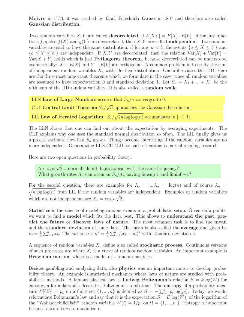
Two random variables X, Y are called decorrelated, if E[XY ] = E[X ] · E[Y ]. If for any func-tions f, g also f(X) and g(Y ) are decorrelated, then X, Y are called independent. Two randomvariables are said to have the same distribution, if for any a < b, the events a ≤ X ≤ b anda ≤ Y ≤ b are independent. If X, Y are decorrelated, then the relation Var[X ] + Var[Y ] =Var[X + Y ] holds which is just Pythagoras theorem, because decorrelated can be understoodgeometrically: X − E[X ] and Y − E[Y ] are orthogonal. A common problem is to study the sumof independent random variables Xn with identical distribution. One abbreviates this IID. Hereare the three most important theorems which we formulate in the case, whee all random variablesare assumed to have expectatation 0 and standard deviation 1. Let Sn = X1 + ... + Xn be then’th sum of the IID random variables. It is also called a random walk.
LLN Law of Large Numbers assures that Sn/n converges to 0.
CLT Central Limit Theorem:Sn/√n approaches the Gaussian distribution.
LIL Law of Iterated Logarithm: Sn/√
2n log log(n) accumulates in [−1, 1].
The LLN shows that one can find out about the expectation by averaging experiments. TheCLT explains why one sees the standard normal distribution so often. The LIL finally gives usa precise estimate how fast Sn grows. Things become interesting if the random variables are nomore independent. Generalizing LLN,CLT,LIL to such situations is part of ongoing research.
Here are two open questions in probability theory:
Are π, e,√2... normal: do all digits appear with the same frequency?
What growth rates Λn can occur in Sn/Λn having limsup 1 and liminf −1?
For the second question, there are examples for Λn = 1, λn = log(n) and of course λn =√
n log log(n) from LIL if the random variables are independent. Examples of random variables
which are not independent are Xn = cos(n√2).
Statistics is the science of modeling random events in a probabilistic setup. Given data points,we want to find a model which fits the data best. This allows to understand the past, pre-dict the future or discover laws of nature. The most common task is to find the mean
and the standard deviation of some data. The mean is also called the average and given bym = 1
n
∑
n
k=1 xk. The variance is σ2 = 1n
∑
n
k=1(xk −m)2 with standard deviation σ.
A sequence of random variables Xn define a so called stochastic process. Continuous versionsof such processes are where Xt is a curve of random random variables. An important example isBrownian motion, which is a model of a random particles.
Besides gambling and analyzing data, also physics was an important motor to develop proba-bility theory. An example is statistical mechanics where laws of nature are studied with prob-abilistic methods. A famous physical law is Ludwig Boltzmann’s relation S = k log(W ) forentropy, a formula which decorates Boltzmann’s tombstone. The entropy of a probability mea-sure P [k] = pk on a finite set 1, ..., n is defined as S = −∑n
i=1 pi log(pi). Today, we wouldreformulate Boltzmann’s law and say that it is the expectation S = E[log(W )] of the logarithm ofthe ”Wahrscheinlichkeit” random variable W (i) = 1/pi on Ω = 1, ..., n . Entropy is importantbecause nature tries to maximize it

E-320: Teaching Math with a Historical Perspective Oliver Knill, 2010-2015
Lecture 9: Topology
Topology studies properties of geometric objects which do not change under continuous reversibledeformations. For a topologist, a coffee cup with 1 handle is the same as a doughnut. One candeform one into the other without punching any holes in it or ripping things apart. Similarly, aplate and a croissant are the same. But a croissant is not equivalent to a bagle. On a bagle, thereare closed curves which can not be deformed to a point. For a topologist the letters O and P are thesame but different from the letter B. The mathematical setup is beautiful: a topological space
is a set X with a set O of subsets of X containing both ∅ and X such that finite intersections andarbitrary unions in O are in O. Sets in O are called open sets and O is called a topology. Thecomplement of an open set is called closed. Examples of topologies are the trivial topology
O = ∅, X , where no open sets besides the empty set and X exist or the discrete topologyO = A ⊂ X ,, where every subset is open. But these are in general not interesting. Animportant example on the plane X is the collection O of sets U in the plane X for which everypoint is the center of a small disc still contained in U . A special class of topological spaces aremetric spaces, where a set X is equipped with a distance function d(x, y) = d(y, x) ≥ 0 whichsatisfies the triangle inequality d(x, y)+d(y, z) ≥ d(x, z) and for which d(x, y) = 0 if and only ifx = y. A set U in a metric space is open if to every x in U , there is a ball Br(x) = y|d(x, y) < r of positive radius r contained in U . Metric spaces are topological spaces but not all topologicalspaces are metric: the trivial topology for example is not in general. For doing calculus on atopological space X , each point has a neighborhood called chart which is topologically equivalentto a disc in Euclidean space. Finitely many such neighborhoods covering X form an atlas of X . Ifthe charts are glued together with identification maps on the intersection one obtains a manifold.Two dimensional examples are the sphere, the torus, the projective plane or the Klein bottle.Topological spaces X, Y are called homeomorphic meaning ”topologically equivalent” if thereis an invertible map from X to Y which is also induces an invertible map on the correspondingtopologies. A basic task is to decide whether two spaces are equivalent in this sense or not. Thesurface of the coffee cup for example is equivalent in this sense to the surface of a doughnut butit is not equivalent to the surface of a sphere.Many properties of geometric spaces can be understood by replacing them with graphs forming askeleton of the space. A graph is a finite collection of vertices V together with a finite set of edgesE, where each edge connects two points in V . For example, the set V of cities in the US where theedges are pairs of cities connected by a street is a graph. The Konigsberg bridge problem wasa trigger puzzle for the study of graph theory. Polyhedra were an other start in graph theory.It study is losely related to the analysis of surfaces. The reason is that one can see polyhedraas discrete versions of surfaces. In computer graphics for example, surfaces are rendered as finitegraphs, using triangularizations.The Euler characteristic of a convex polyhedron is a remarkable topological invariant. It is
V − E + F = 2 , where V is the number of vertices, E the number of edges
and F the number of faces. This number is equal to 2 for connected polyhedra in which everyclosed loop can be pulled together to a point. This formula for the Euler characteristic is also calledEuler’s gem, a fact which comes with a rich history. Rene Descartes seems have stumbledupon it and written it down in a secret notebook. It was Leonard Euler in 1752 was the first toproved the formula for convex polyhedra. A convex polyhedron is called a platonic solid, if allvertices are on the unit sphere, all edges have the same length and all faces are congruent polygons.A theorem of Theaetetus states that there are only 5 platonic solids: [Proof: Assume the faces

are regular n-gons and m of them meet at each vertex. Beside the Euler relation V +E + F = 2,a polyhedron also satisfies the relations nF = 2E and mV = 2E which are obvious from countingvertices or edges in different ways. This gives 2E/m−E + 2E/n = 2 or 1/n+ 1/m = 1/E +1/2.From n ≥ 3 and m ≥ 3 we see that it is impossible that both m and n are larger than 3. Thereare now nly two possibilities: either n = 3 or m = 3. In the case n = 3 we have m = 3, 4, 5 inthe case m = 3 we have n = 3, 4, 5. The five possibilities (3, 3), (3, 4), (3, 5), (4, 3), (5, 3) representthe 5 platonic solids.] The pairs (n,m) are called the Schlafly symbol of the polyhedron:
Name V E F V-E+F Schlaflitetrahedron 4 6 4 2 3, 3hexahedron 8 12 6 2 4, 3octahedron 6 12 8 2 3, 4
Name V E F V-E+F Schlafli
dodecahedron 20 30 12 2 5, 3icosahedron 12 30 20 2 3, 5
The Greeks proved this more geometrically: Euclid showed in his ”Elements” that at each vertex,we can attach 3,4 or 5 equilateral triangles, 3 squares or 3 regular pentagons. (6 triangles, 4squares or 4 pentagons would lead to a total angle which is too large because each corner musthave at least 3 different edges). Simon Antoine-Jean L’Huilier refined in 1813 Euler’s formula
to situations with holes: V − E + F = 2− 2g , where g is the number of holes. For adoughnut with one hole we have V − E + F = 0. . Cauchy first proved that there are exactly 4non-convex regular Kepler-Poinsot polyhedra. Their Euler characteristic can be different.
Name V E F V-E+F Schlaflismall stellated dodecahedron 12 30 12 -6 5/2, 5great dodecahedron 12 30 12 -6 5, 5/2great stellated dodecahedron 20 30 12 2 5/2, 3great icosahedron 12 30 20 2 3, 5/2
If two different face types are allowed but each vertex still look the same, one obtains 13 semi-
regular polyhedra. They were first studied by Archimedes in 287 BC. Since his work is lost,Johannes Kepler is considered the first person since antiquity to describe the whole set of thir-teen in his ”Harmonices Mundi”. The Euler characteristic χ = 2 − 2g is also useful for surfaces.One can reduce the question to graphs, triangularizations of the surface. The Euler characteristiccompletely characterizes smooth compact surfaces if they are orientable. A non-orientable surface,the Klein bottle can be obtained by gluing ends of the Mobius strip. Classifying higher dimen-sional manifolds is more difficult and finding more invariants is part of modern research. Higheranalogues of polyhedra are called polytopes (Alicia Boole Stott). Regular polytopes are theanalogue of the platonic solids in higher dimensions. Here they are for the first few dimensions:
dimension name Schlafli symbols2: Regular polygons 3, 4, 5, ...3: Platonic solids 3, 3, 3, 4, 3, 5, 4, 3, 5, 34: Regular 4D polytopes 3, 3, 3, 4, 3, 3, 3, 3, 4, 3, 4, 3, 5, 3, 3, 3, 3, 5≥ 5: Regular polytopes 3, 3, 3, . . . , 3, 4, 3, 3, . . . , 3, 3, 3, 3, . . . , 3, 4
Ludwig Schlafly found in 1852 that there are exactly six convex regular convex 4-polytopes orpolychora. The expression ”choros” is Greek for ”space”. Schlaefli’s polyhedral formula tells thatfor any convex polytope in four dimensions, the relation V − E + F − C = 0 holds,where C is the number of 3-dimensional chambers. In dimensions 5 and higher, there are only3 types of polytopes: the higher dimensional analogues of the tetrahedron, octahedron and the
cube. A general formula∑
d−1
i=0(−1)iVi = 1− (−1)d gives the Euler characteristic of a convex
polytop in d dimensions with i-dimensional parts Vi.

E-320: Teaching Math with a Historical Perspective Oliver Knill, 2010-2015
Lecture 10: Analysis
Analysis is the science of measure and optimization. As a collection of mathematical fields, itcontains real and complex analysis, functional analysis, harmonic analysis and calculus
of variations. Analysis has relations to calculus, geometry, topology, probability theory anddynamics. We will focus mostly on ”the geometry of fractals” today. Examples are Julia setswhich belong to the subfield of ”complex analysis” of ”dynamical systems”. ”Calculus of varia-tions” is illustrated by the Kakeya needle set in ”geometric measure theory”, a glimpse of ”Fourieranalysis” is seen by looking at functions which have fractal graphs, ”spectral theory” as part offunctional analysis is represented by the ”Hofstadter butterfly”. As we take a tabloid approachand describe the topic with gossip about some ”pop icons” in each field, consider this page thecenter fold page of the ”Analytical Enquirer”.
A fractal is a set with non-integer dimension. An example is the Cantor set, as discoveredin 1875 by Henry Smith. Start with the unit interval. Cut the middle third, then cut themiddle third from both parts then the middle parts of the four parts etc. The limiting set is theCantor set. The mathematical theory of fractals belongs to measure theory and can also bethought of a playground for real analysis or topology. The term fractal had been introduced byBenoit Mandelbrot in 1975. Dimension can be defined in different ways. The simplest is the box
counting definition which works for most household fractals: if we need n squares of length
r to cover a set, then d = − log(n)/ log(r) converges to the dimension of the set with
r → 0. A curve of length L for example needs L/r squares of length r so that its dimensionis 1. A region of area A needs A/r2 squares of length r to be covered and its dimension is 2.The Cantor set needs to be covered with n = 2m squares of length r = 1/3m. Its dimension is− log(n)/ log(r) = −m log(2)/(m log(1/3)) = log(2)/ log(3).Examples of fractals (for the first, the dimension is not yet known):
Weierstrass function 1872Koch snowflake 1904Sierpinski carpet 1915Menger sponge 1926
0.2 0.4 0.6 0.8 1.0
-0.5
0.5
1.0
Complex analysis extends calculus to the complex. It deals with functions f(z) defined in thecomplex plane. Integration is done along paths. Complex analysis completes the understand-ing about functions. It also provides more examples of fractals by iterating functions like thequadratic map f(z) = z2 + c:
Newton method 1879Julia sets 1918Mandelbrot set 1978Mandelbar set 1989
Particularly famous are the Douady rabbit and the dragon, the dendrite, the airplane.Calculus of variations is calculus in infinite dimensions. Taking derivatives is called taking”variations”. Historically, it started with the problem to find the curve of fastest fall leading tothe Brachistochrone r(t) = (t− sin(t), 1− cos(t)). In calculus, we find maxima and minima offunctions. In calculus of variations, we extremize on much larger spaces. Here are some examplesof problems:

Brachistochrone 1696Minimal surface 1760Geodesics 1830Isoperimetric problem 1838Kakeya Needle problem 1917
Start
Fourier theory decomposes a function into basic components of various frequencies f(x) =a1 sin(x) + a2 sin(2x) + a3 sin(3x)... . The numbers ai are called Fourier coefficients. Our eardoes such a decomposition, when we listen to music. By distinguish different frequencies, our earproduces a Fourier analysis.
Fourier series 1729Fourier transform (FT) 1811Discrete FT Gauss?Wavelet transform 1930
-3 -2 -1 1 2 3
-0.2
0.2
0.4
0.6
0.8
1.0
The Weierstrass function mentioned above is given as the Fourier series∑
n an cos(πbnx) with
0 < a < 1, ab > 1 + 3π/2. The dimension of its graph is believed to be 2 + log(a)/ log(b).Spectral theory analyzes linear maps L. The spectrum are the real numbers E such thatL−E is not invertible. A Hollywood celebrity among all linear maps is the Matthieu operator
L(x)n = xn+1+xn−1+(2− 2 cos(cn))xn: if we draw the spectrum for for each c, we see the Hofs-
tadter butterfly. For fixed c the map describes the behavior of an electron in an almost periodiccrystal. An other famous system is the quantum harmonic oscillator, L(f) = f ′′(x) + f(x),the vibrating drum L(f) = fxx + fyy, where f is the amplitude of the drum and f = 0 on theboundary of the drum.
Hydrogen atom 1914Hofstadter butterfly 1976Harmonic oscillator 1900Vibrating drum 1680
+
-
All these examples in analysis look unrelated at first. Fractal geometry ties many of them together:spectra are often fractals, minimal configurations have fractal nature, like in solid state physics orin diffusion limited aggregation or in other critical phenomena like percolation phenomena,cracks in solids or the formation of lighting bolts In Hamiltonian mechanics, minimal energyconfigurations are often fractals like Mather theory. And solutions to minimizing problems leadto fractals in a natural way like when you have the task to turn around a needle on a table by 180degrees and minimize the area swept out by the needle. The minimal turn leads to a Kakaya set,which is a fractal. Finally, lets mention some unsolved problems in analysis: does the Riemann
zeta function f(z) =∑
∞
n=1 1/nz have all nontrivial roots on the axis Re(z) = 1/2? This question
is called the Riemann hypothesis and is the most important open problem in mathematics. Itis an example of a question in analytic number theory which also illustrates how analysis hasentered into number theory. Some mathematicians think that spectral theory might solve it. Alsothe Mandelbrot set M is not understood yet: the ”holy grail” in the field of complex dynamics isthe problem whether it M is locally connected. From the Hofstadter butterfly one knows that ithas measure zero. What is its dimension? An other open question in spectral theory is the ”canone hear the sound of a drum” problem which asks whether there are two convex drums whichare not congruent but which have the same spectrum. In the area of calculus of variations, justone problem: how long is the shortest curve in space such that its convex hull (the union of allpossible connections between two points on the curve) contains the unit ball.

E-320: Teaching Math with a Historical Perspective Oliver Knill, 2010-2015
Lecture 11: Cryptography
Cryptography is the theory of codes. Two important aspects of the field are the encryption
rsp. decryption of information and error correction. Both are crucial in daily life. Whengetting access to a computer, viewing a bank statement or when taking money from the ATM,encryption algorithms are used. When phoning, surfing the web, accessing data on a computeror listening to music, error correction algorithms are used. Since our lives have become more andmore digital: music, movies, books, journals, finance, transportation, medicine, and communi-cation have become digital, we rely on strong error correction to avoid errors and encryption toassure things can not be tempered with. Without error correction, airplanes would crash: smallerrors in the memory of a computer would produce glitches in the navigation and control program.In a computer memory every hour a couple of bits are altered, for example by cosmic rays. Errorcorrection assures that this gets fixed. Without error correction music would sound like a 1920gramophone record. Without encryption, everybody could intrude electronic banks and transfermoney. Medical history shared with your doctor would all be public. Before the digital age, errorcorrection was assured by extremely redundant information storage. Writing a letter on a pieceof paper displaces billions of billions of molecules in ink. Now, changing any single bit could givea letter a different meaning. Before the digital age, information was kept in well guarded safeswhich were physically difficult to penetrate. Now, information is locked up in computers whichare connected to other computers. Vaults, money or voting ballots are secured by mathematicalalgorithms which assure that information can only be accessed by authorized users. Also lifeneeds error correction: information in the genome is stored in a genetic code, where a errorcorrection makes sure that life can survive. A cosmic ray hitting the skin changes the DNA ofa cell, but in general this is harmless. Only a larger amount of radiation can render cells cancerous.
How can an encryption algorithm be safe? One possibility is to invent a new method and keep itsecret. An other is to use a well known encryption method and rely on the difficulty of mathe-
matical computation tasks to assure that the method is safe. History has shown that the firstmethod is unreliable. Systems which rely on ”security through obfuscation” usually do not last.The reason is that it is tough to keep a method secret if the encryption tool is distributed. Reverseengineering of the method is often possible, for example using plain text attacks. Given a mapT , a third party can compute pairs x, T (x) and by choosing specific texts figure out what happens.
The Caesar cypher permutes the letters of the alphabet. We can for example replace every letterA with B, every letter B with C and so on until finally Z is replaced with A. The word ”Math-ematics” becomes so encrypted as ”Nbuifnbujdt”. Caesar would shift the letters by 3. The rightshift just discussed was used by his Nephew Augustus. Rot13 shifts by 13, and Atbash cypher
reflects the alphabet, switch A with Z, B with Y etc. The last two examples are involutive: en-cryption is decryption. More general cyphers are obtained by permuting the alphabet. Because of26! = 403291461126605635584000000 ∼ 1027 permutations, it appears first that a brute force at-tack is not possible. But Cesar cyphers can be cracked very quickly using statistical analysis. If weknow the frequency with which letters appear and match the frequency of a text we can figure outwhich letter was replaced with which. The Trithemius cypher prevents this simple analysis bychanging the permutation in each step. It is called a polyalphabetic substitution cypher. Insteadof a simple permutation, there are many permutations. After transcoding a letter, we also changethe key. Lets take a simple example. Rotate for the first letter the alphabet by 1, for the second

letter, the alphabet by 2, for the third letter, the alphabet by 3 etc. The word ”Mathematics” be-comes now ”Ncwljshbrmd”. Note that the second ”a” has been translated to something differentthan a. A frequency analysis is now more difficult. The Viginaire cypher adds even more com-plexity: instead of shifting the alphabet by 1, we can take a key like ”BCNZ”, then shift the firstletter by 1, the second letter by 3 the third letter by 13, the fourth letter by 25 the shift the 5thletter by 1 again. While this cypher remained unbroken for long, a more sophisticated frequencyanalysis which involves first finding the length of the key makes the cypher breakable. With theemergence of computers, even more sophisticated versions like the German enigma had no chance.
Diffie-Hellman key exchange allows Ana and Bob want to agree on a secret key over a publicchannel. The two palindromic friends agree on a prime number p and a base a. This informationcan be exchanged publically. Ana choses now a secret number x and sends X = ax modulo p
to Bob over the channel. Bob choses a secret number y and sends Y = ay modulo p to Ana.Ana can compute Y x and Bob can compute Xy but both are equal to axy. This number is theircommon secret. The key point is that eves dropper Eve, can not compute this number. The onlyinformation available to Eve are X and Y , as well as the base a and p. Eve knows that X = ax
but can not determine x. The key difficulty in this code is the discrete log problem: getting x
from ax modulo p is believed to be difficult for large p.The Rivest-Shamir-Adleman public key system uses a RSA public key (n, a) with aninteger n = pq and a < (p− 1)(q − 1), where p, q are prime. Also here, n and a are public. Onlythe factorization of n is kept secret. Ana publishes this pair. Bob who wants to email Ana amessage x, sends her y = xa mod n. Ana, who has computed b with ab = 1 mod (p−1)(q−1) canread the secrete email y because yb = xab = x(p−1)(q−1) = x modn. But Eve, has no chance becausethe only thing Eve knows is y and (n, a). It is believed that without the factorization of n, itis not possible to determine x. The message has been transmitted securely. The core difficulty isthat taking roots in the ring Zn = 0, . . . , n− 1 is difficult without knowing the factorizationof n. With a factorization, we can quickly take arbitrary roots. If we can take square roots, thenwe can also factor: assume we have a product n = pq and we know how to take square roots of 1.If x solves x2 = 1 mod n and x is different from 1, then x2 − 1 = (x− 1)(x+ 1) is zero modulo n.This means that p divides (x− 1) or (x+ 1). To find a factor, we can take the greatest commondivisor of n, x − 1. Take n = 77 for example. We are given the root 34 of 1. ( 342 = 1156 hasreminder 1 when divided by 34). The greatest common divisor of 34−1 and 77 is 11 is a factor of77. Similarly, the greatest common divisor of 34+ 1 and 77 is 7 divides 77. Finding roots moduloa composite number and factoring the number is equally difficult.
Cipher Used for Difficulty AttackCesar transmitting messages many permutations StatisticsViginere transmitting messages many permutations StatisticsEnigma transmitting messages no frequency analysis Plain textDiffie-Helleman agreeing on secret key discrete log mod p Unsafe primesRSA electronic commerce factoring integers Factoring
The simplest error correcting code uses 3 copies of the same information. A single error canbe corrected. With 3 watches for example, you know the time even if one of the watches fails.Cockpits of airplanes have three copies important instruments. But this basic error correctingcode is not efficient. It can correct single errors by tripling the size. Its efficiency is 33 percent.A cheap way to make it more efficient is to compress the data first and then make three copies.Data compression is a topic by itself. Here is a simple example, the dictionary compression.Take dictionary with 65′536 = 216 words for example. Every word can be encode by two bytes.Assuming an average word length of 6, we can encode every word with 2 bytes instead of 6. Thereare better error correcting codes using linear algebra or algebraic geometry.

E-320: Teaching Math with a Historical Perspective Oliver Knill, 2010-2015
Lecture 12: Dynamical systems
Dynamical systems theory is the science of time evolution. If time is continuous the evo-lution is defined by a differential equation x = f(x). If time is discrete then we look at theiteration of a map x → T (x).
The goal is to predict the future of the system when the present state is known. A differential
equation is an equation of the form d/dtx(t) = f(x(t)), where the unknown quantity is a pathx(t) in some “phase space”. We know the velocity d/dtx(t) = x(t) at all times and the initialconfiguration x(0)), we can to compute the trajectory x(t). What happens at a future time?Does x(t) stay in a bounded region or escape to infinity? Which areas of the phase space arevisited and how often? Can we reach a certain part of the space when starting at a given pointand if yes, when. An example of such a question is to predict, whether an asteroid located at a spe-cific location will hit the earth or not. An other example is to predict the weather of the next week.
An examples of a dynamical systems in one dimension is the differential equation
x′(t) = x(t)(2− x(t)), x(0) = 1
It is called the logistic system and describes population growth. This system has the solutionx(t) = 2et/(1 + e2t) as you can see by computing the left and right hand side.
A map is a rule which assigns to a quantity x(t) a new quantity x(t + 1) = T (x(t)). The statex(t) of the system determines the situation x(t + 1) at time t + 1. An example is is the Ulam
map T (x) = 4x(1 − x) on the interval [0, 1]. This is an example, where we have no idea whathappens after a few hundred iterates even if we would know the initial position with the accuracyof the Planck scale.
Dynamical system theory has applications all fields of mathematics. It can be used to find rootsof equations like for
T (x) = x− f(x)/f ′(x) .
A system of number theoretical nature is the Collatz map
T (x) =x
2(evenx), 3x+ 1 else .
A system of geometric nature is the Pedal map which assigns to a triangle the pedal triangle.
About 100 years ago, Henry Poincare was able to deal with chaos of low dimensional systems.While statistical mechanics had formalized the evolution of large systems with probabilisticmethods already, the new insight was that simple systems like a three body problem or abilliard map can produce very complicated motion. It was Poincare who saw that even forsuch low dimensional and completely deterministic systems, random motion can emerge. Whilephysisists have dealt with chaos earlier by assuming it or artificially feeding it into equations likethe Boltzmann equation, the occurrence of stochastic motion in geodesic flows or billiards orrestricted three body problems was a surprise. These findings needed half a century to sink inand only with the emergence of computers in the 1960ies, the awakening happened. Icons like

wing of a butterfly can produce a tornado in Texas in a few weeks. The reason for this statementis that the complicated equations to simulate the weather reduce under extreme simplificationsand truncations to a simple differential equation x = σ(y − x), y = rx− y − xz, z = xy − bz, theLorenz system. For σ = 10, r = 28, b = 8/3, Ed Lorenz discovered in 1963 an interesting longtime behavior and an aperiodic ”attractor”. Ruelle-Takens called it a strange attractor. It is agreat moment in mathematics to realize that attractors of simple systems can become fractalson which the motion is chaotic. It suggests that such behavior is abundant. What is chaos? If adynamical system shows sensitive dependence on initial conditions, we talk about chaos.We will experiment with the two maps T (x) = 4x(1−x) and S(x) = 4x−4x2 which starting withthe same initial conditions will produce different outcomes after a couple of iterations.The sensitive dependence on initial conditions is measured by how fast the derivative dT n of then’th iterate grows. The exponential growth rate γ is called the Lyapunov exponent. A smallerror of the size h will be amplified to heγn after n iterates. In the case of the Logistic map withc = 4, the Lyapunov exponent is log(2) and an error of 10−16 is amplified to 2n · 10−16. For timen = 53 already the error is of the order 1. This explains the above experiment with the differentmaps. The maps T (x) and S(x) round differently on the level 10−16. After 53 iterations, theseinitial fluctuation errors have grown to a macroscopic size.Here is a famous open problem which has resisted many attempts to solve it: Show that the mapT (x, y) = (c sin(2πx) + 2x − y, x) with T n(x, y) = (fn(x, y), gn(x, y)) has sensitive dependenceon initial conditions on a set of positive area. More precisely, verify that for c > 2 and all n1
n
∫1
0
∫1
0log |∂xfn(x, y)| dxdy ≥ log( c
2). The left hand side converges to the average of the Lyapunov
exponents which is in this case also the entropy of the map. For some systems, one can computethe entropy. The logistic map with c = 4 for example, which is also called the Ulam map, hasentropy log(2). The cat map
T (x, y) = (2x+ y, x+ y) mod1
has entropy log |(√5 + 3)/2|. This is the logarithm of the larger eigenvalue of the matrix.
While questions about simple maps look artificial at first, the mechanisms prevail in other systems:in astronomy, when studying planetary motion or electrons in the van Allen belt, in mechanicswhen studying coupled penduli or nonlinear oscillators, in fluid dynamics when studying vortexmotion or turbulence, in geometry, when studying the evolution of light on a surface, the change ofweather or tsunamis in the ocean. Dynamical systems theory started historically with the problemto understand the motion of planets. Newton realized that this is governed by a differentialequation, the n-body problem
x′′
j (t) =n∑
i=1
cij(xi − xj)
|xi − xj |3,
where cij depends on the masses and the gravitational constant. If one body is the sun andno interaction of the planets is assumed and using the common center of gravity as the origin,this reduces to the Kepler problem x′′(t) = −Cx/|x|3, where planets move on ellipses, theradius vector sweeps equal area in each time and the period squared is proportional to the semi-major axes cubed. A great moment in astronomy was when Kepler derived these laws empirically.An other great moment in mathematics is Newton’s theoretically derivation from the differentialequations.
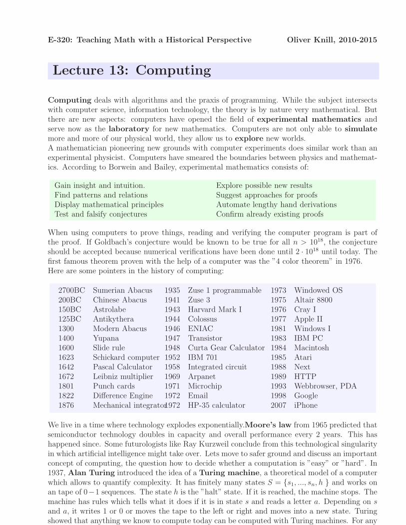
E-320: Teaching Math with a Historical Perspective Oliver Knill, 2010-2015
Lecture 13: Computing
Computing deals with algorithms and the praxis of programming. While the subject intersectswith computer science, information technology, the theory is by nature very mathematical. Butthere are new aspects: computers have opened the field of experimental mathematics andserve now as the laboratory for new mathematics. Computers are not only able to simulate
more and more of our physical world, they allow us to explore new worlds.A mathematician pioneering new grounds with computer experiments does similar work than anexperimental physicist. Computers have smeared the boundaries between physics and mathemat-ics. According to Borwein and Bailey, experimental mathematics consists of:
Gain insight and intuition.Find patterns and relationsDisplay mathematical principlesTest and falsify conjectures
Explore possible new resultsSuggest approaches for proofsAutomate lengthy hand derivationsConfirm already existing proofs
When using computers to prove things, reading and verifying the computer program is part ofthe proof. If Goldbach’s conjecture would be known to be true for all n > 1018, the conjectureshould be accepted because numerical verifications have been done until 2 · 1018 until today. Thefirst famous theorem proven with the help of a computer was the ”4 color theorem” in 1976.Here are some pointers in the history of computing:
2700BC Sumerian Abacus200BC Chinese Abacus150BC Astrolabe125BC Antikythera1300 Modern Abacus1400 Yupana1600 Slide rule1623 Schickard computer1642 Pascal Calculator1672 Leibniz multiplier1801 Punch cards1822 Difference Engine1876 Mechanical integrator
1935 Zuse 1 programmable1941 Zuse 31943 Harvard Mark I1944 Colossus1946 ENIAC1947 Transistor1948 Curta Gear Calculator1952 IBM 7011958 Integrated circuit1969 Arpanet1971 Microchip1972 Email1972 HP-35 calculator
1973 Windowed OS1975 Altair 88001976 Cray I1977 Apple II1981 Windows I1983 IBM PC1984 Macintosh1985 Atari1988 Next1989 HTTP1993 Webbrowser, PDA1998 Google2007 iPhone
We live in a time where technology explodes exponentially.Moore’s law from 1965 predicted thatsemiconductor technology doubles in capacity and overall performance every 2 years. This hashappened since. Some futurologists like Ray Kurzweil conclude from this technological singularityin which artificial intelligence might take over. Lets move to safer ground and discuss an importantconcept of computing, the question how to decide whether a computation is ”easy” or ”hard”. In1937, Alan Turing introduced the idea of a Turing machine, a theoretical model of a computerwhich allows to quantify complexity. It has finitely many states S = s1, ..., sn, h and works onan tape of 0−1 sequences. The state h is the ”halt” state. If it is reached, the machine stops. Themachine has rules which tells what it does if it is in state s and reads a letter a. Depending on s
and a, it writes 1 or 0 or moves the tape to the left or right and moves into a new state. Turingshowed that anything we know to compute today can be computed with Turing machines. For any

known machine, there is a polynomial p so that a computation done in k steps with that computercan be done in p(k) steps on a Turing machine. What can actually be computed? Church’s thesisof 1934 states that everything which can be computed can be computed with Turing machines.Similarly as in mathematics itself, there are limitations of computing. Turing’s setup allowed himto enumerate all possible Turing machine and use them as input of an other machine. Denote byTM the set of all pairs (T, x), where T is a Turing machine and x is a finite input. Let H ⊂ TM
denote the set of Turing machines (T, x) which halt with the tape x as input. Turing looked atthe decision problem: is there a machine which decides whether a given machine (T, x) is in H ornot. An ingenious Diagonal argument of Turing shows that the answer is ”no”. [Proof: assumethere is a machine HALT which returns from the input (T, x) the output HALT(T, x) = true, ifT halts with the input x and otherwise returns HALT(T, x) = false. Turing constructs a Turingmachine DIAGONAL, which does the following:
1) Read x. 2) Define Stop=HALT(x,x) 3) While Stop=True repeat Stop:=True; 4) Stop
Now, DIAGONAL is either in H or not. If DIAGONAL is in H, then the variable Stop is truewhich means that the machine DIAGONAL runs for ever and DIAGONAL is not in H. But ifDIAGONAL is not in H, then the variable Stop is false which means that the loop 3) is neverentered and the machine stops. The machine is in H.]Lets go back to the problem of distinguishing ”easy” and ”hard” problems: One calls P theclass of decision problems that are solvable in polynomial time and NP the class of decisionproblems which can efficiently be tested if the solution is given. These categories do not dependon the computing model used. The question ”N=NP?” is the most important open problem intheoretical computer science. It is one of the seven millenium problems and it is widely believedthat P 6= NP . If a problem is such that every other NP problem can be reduced to it, it is calledNP-complete. Popular games like Minesweeper or Tetris are NP-complete. If P 6= NP , thenthere is no efficient algorithm to beat the game. The intersection of NP-hard and NP is the classof NP-complete problems. An example of an NP-complete problem is the balanced number
partitioning problem: given n positive integers, divide them into two subsets A,B, so that thesum in A and the sum in B are as close as possible. A first shot: chose the largest remainingnumber and distribute it to alternatively to the two sets.We all feel that it is harder to find a solution to a problem rather than to verify a solution.If N 6= NP there are one way functions, functions which are easy to compute but hard to verify.For some important problems, we do not even know whether they are in NP. Here are two examples:1) the integer factoring problem: given n find the factors 2) the merit factor problem:minimize
∑nk=−n c
2k, where ck =
∑n−kj=0 ajaj+k An efficient algorithm for the first one would have
enormous consequences for ou modern lives.Finally, lets look at some mathematical problems in artificial intelligence AI:
problem solving playing games like chess, performing algorithms, solving puzzlespattern matching speech, music, image, face, handwriting, plagiarism detection, spamreconstruction tomography, city reconstruction, body scanningresearch computer assisted proofs, discovering theorems, verifying proofsdata mining knowledge acquisition, knowledge organization, learningtranslation language translation, porting applications to programming languagescreativity writing poems, jokes, novels, music pieces, painting, sculpturesimulation physics engines, evolution of bots, game development, aircraft designinverse problems earth quake location, oil depository, tomographyprediction weather prediction, climate change, warming, epidemics, supplies
We had started with basic human activities defining mathematical fields, we end the course withmathematical activities defining some aspects of computing. Our journey through math is over.