Lecture 1: Common measures for dependability evaluation ...

Lecture 1: Common measures for dependability evaluation

Viacheslav “Slava” Izosimov Safety-Critical Systems Competence Center Semcon Sweden AB 18 September 2013

Lecture 2: Design optimization for fault tolerant distributed embedded systems

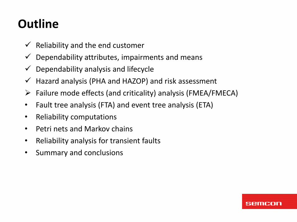
Outline Reliability and the end customer • Dependability attributes, impairments and means • Dependability analysis and lifecycle • Hazard analysis (PHA and HAZOP) and risk assessment • Failure mode effects (and criticality) analysis (FMEA/FMECA) • Fault tree analysis (FTA) and event tree analysis (ETA) • Reliability computations • Petri nets and Markov chains • Reliability analysis for transient faults • Summary and conclusions

Robustness and the end customer

• Functions – often #1 • BUT… functions have to function • If they don’t, …

• Complex function – high value – reduction in reliability • Simple function – low value – high reliability

• The question is what to choose?

• Avionics: a simple function is preferred and requirements

on reliability are very stringent • Consumer electronics: complexity may increase, and, with

greater complexity, higher fault rate and greater need for robust designs!

Outline Reliability and the end customer Dependability attributes, impairments and means • Dependability analysis and lifecycle • Hazard analysis (PHA and HAZOP) and risk assessment • Failure mode effects (and criticality) analysis (FMEA/FMECA) • Fault tree analysis (FTA) and event tree analysis (ETA) • Reliability computations • Petri nets and Markov chains • Reliability analysis for transient faults • Summary and conclusions

Dependability attributes

dependability

availability reliability safety integrity maintainability

attributes

Terminology is based on A. Avizienis, J.-C. Laprie, B. Randell, and C. Landwehr “Basic Concepts and Taxonomy of Dependable and Secure Computing”, IEEE Trans. on Dependable and Secure Computing, 1(1), 2004.

Dependability: is the ability of a system to deliver its intended level of service to its users

Where is security? confidentiality

security attributes

Dependability attributes • Availability: readiness for correct service

– Highly available systems: telecom, < 5 min./year unavailable • Reliability: continuity of correct service

– Highly reliable systems: airplane, R(several hours) = 0.999 999 9 = 0.97 • Safety: absence of catastrophic consequences on the user(s) and the

environment – Highly safe system: railway signalling with all semaphores red

• Integrity: absence of improper system alterations – System with high integrity: high-quality Swiss watches

• Maintainability: ability to undergo modifications and repairs – Highly maintainable system: a chassis with “hot plug” components

Dependability impairments: fault, error and failure

Fault Error Failure Fault

Error detection

Fault tolerance

Subsystem A of System B (Semaphore subsystem of

a train transportation system)

System B (Train transportation system)

“0” “1”

Error Failure

“STOP”

“GO”

Error detection

Fault tolerance

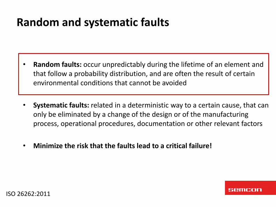
Random and systematic faults

• Random faults: occur unpredictably during the lifetime of an element and that follow a probability distribution, and are often the result of certain environmental conditions that cannot be avoided

• Systematic faults: related in a deterministic way to a certain cause, that can only be eliminated by a change of the design or of the manufacturing process, operational procedures, documentation or other relevant factors

• Minimize the risk that the faults lead to a critical failure!

ISO 26262:2011

Classification in terms of persistence

Transient faults

Happen for a short time and disappear

Do not cause a permanent damage of circuits

Corruptions of data, miscalculation in logic

Intermittent faults Manifest in the same way as

transient faults Happen repeatedly Disappear and, then, re-

appear after some time

Permanent faults Happen and stay Cause a permanent damage Repair is necessary

N. Storey, “Safety-Critical Computer Systems”, Addison-Wesley, 1996.

Few more…

• Timing faults (glitches)

• Omission faults

– Wrong results stay inside and “never” passed…

• Byzantine faults – The most general faults: may appear in any

unpredictable way

• Latent (dormant) faults

Aging - Bath curve

Installation / production End of life (aging)

Some causes of random faults

Loose connectors

Aging

Crosstalk

Power supply fluctuations

Internal EMI Radiation

Electromagnetic interference (EMI)

Lightning storms Software errors “Heisenbugs”

Dependability means Fault avoidance: prevent the occurrence or introduction of faults Example: to avoid transient faults use an “old” technology with “big” transistors, i.e., use 90nm instead of 32nm.

Fault masking: avoid service failures in the presence of faults Example: to mask transient faults, cross-connect redundant transistors

Fault tolerance: reduce the number and severity of faults Example: to tolerate transient faults on a system level, re-execute processes if the fault occurs

Fault forecasting: estimate the present number, the future incidence, and the likely consequences of faults Example: predict aging processes in a chip to replace the chip before the rate of transient faults becomes dangerously high

Outline Reliability and the end customer Dependability attributes, impairments and means Dependability analysis and lifecycle • Hazard analysis (PHA and HAZOP) and risk assessment • Failure mode effects (and criticality) analysis (FMEA/FMECA) • Fault tree analysis (FTA) and event tree analysis (ETA) • Reliability computations • Petri nets and Markov chains • Reliability analysis for transient faults • Summary and conclusions

Dependability Analyses and Lifecycle System Safety Engineering

Planning

Safety-Critical Systems and Events Identification

Subsystem Hazard Analysis, Risk Assessment

System Hazard Analysis, Risk Assessment

Validation and Verification

Objectives, approaches, scope

Safety-critical systems Safety-critical scenarios and events

Failure modes, effects, mitigating measures

Design-level safety requirements

Reduction of risk to acceptable levels

Source: FAA

Dependability Analyses and Lifecycle Item Definition

Initiation of the safety lifecycle

Hazard Analysis and Risk Assessment

Product Development (System Level)

Software Level

Hardware Level

Release for Production

Production

Operation, service and decommissioning

Other technologies

Controllability

External measures

Operation planning

Production planning

Back to appropriate lifecycle phase

Con

cept

pha

se

Prod

uct

deve

lopm

ent

Afte

r SO

P

Functional Safety Concept

Source: ISO 26262

Dependability Analyses and Lifecycle Source: Agile development

1. Create user story

2. Specify requirements & assumptions

3. Get client approval

4. Groom with Scrum team

5. Schedule into sprint

6. Begin development

7. Sign off internally

8. Conduct user testing

Dependability Analyses and Lifecycle PHA

System FMEA

HAZOP

Software FTA

System ETA System FTA

Functional Tree

Hardware FTA FMECA

Component FMEA

CCF Analyses

Process FMEA

Service FMEA Maintenance FMEA

Hardware ETA

JSA

Maintenance JSA

Markov chains

Reliability Blocks Diagrams

Dependability Failure Analysis

Provide a robust set of qualitative and quantitative evidences

Monte Carlo Sim. HW

Monte Carlo Sim. System

Dependability Analyses and Lifecycle

Item HW

HAZOP

PHA FMEA/FMECA (system)

FTA (system)

FTA (elements)

ETA

Markov chains

Petri nets FMEA (elements)

FMEDA

Monte Carlo Sim.

Dependability Analyses and Lifecycle

Hazard identification

Assessment of risks

Analyses and testing

Propose mitigations / actions

Implement selected measures

Outline Reliability and the end customer Dependability attributes, impairments and means Dependability analysis and lifecycle Hazard analysis (PHA and HAZOP) and risk assessment • Failure mode effects (and criticality) analysis (FMEA/FMECA) • Fault tree analysis (FTA) and event tree analysis (ETA) • Reliability computations • Petri nets and Markov chains • Reliability analysis for transient faults • Summary and conclusions

Hazard Analysis and Risk Assessment

• Hazard Analysis and Risk Assessment (HARA) • Hazard analysis (HA)

– Identification of potential hazards (dangerous situations & events)

– Hazard: a potential source of harm • Risk assessment (RA)

– Assessment of hazards with respects to combination of the probability of occurrence of harm and the severity

– Ranking of hazards according to risks

Hazards are system states combined with certain environmental conditions that cause accidents… They are not faults but faults contribute to hazards…

Preliminary Hazard Analysis (PHA)

• Brainstorming activity to identify initial list of hazards • Using information known about the system so far • Some information is available for the system, some is not… • Usually is ad hoc and is performed at the beginning • Quality depends on the level of experts involved • Creates a basis for further iterations of hazard analysis

Preliminary Hazard Analysis (PHA)

From H2 Refuelling Station concepts, By Norsk Hydro ASA and DNV

Hazard and Operability Study (HAZOP)

• Systematic method to conduct hazard analysis • Allows to go beyond human capability • Relies on pre-defined “keywords” • Expert help is important but even less experienced can

contribute • Conducted in a number of structured HAZOP workshops • Documentation and follow up are important • Time consuming…


• NO (NOT) : Complete negation of the design intent • MORE : Quantitative increase • LESS: Quantitative decrease • AS WELL AS: Qualitative modification/increase • PART OF: Qualitative modification/decrease • REVERSE: Logical opposite of the design intent • OTHER THAN: Complete substitution • EARLY: Relative to the clock time • LATE: Relative to the clock time • BEFORE: Relating to order or sequence • AFTER: Relating to order or sequence


• “Study leader” – workshop moderator • “Recorder” (secretary) • “Designer” • “User” • “Specialist(s)” • “Maintainer”


• Result: – Proving systematic list of deviations with the following

information: • Defining consequences (will be important for RA) • Identifying causes • Defining possible safeguards, simple countermeasures • Defining safety goals • Determining safe states (if possible)


Hazard and operability study – Function: Apply Stimuli to Test Object Guide Word

Deviation Consequences Causes Safeguards Safety Goal Safe State

Other Wrong stimuli applied to the test object

Potential false negative

Communication error. Memory error. Logical error.

Log output to test object. Memory Protection. Logic check. Diversified implementation. Calibration.

Wrong stimuli shall not be applied to the test object

Warning of failure

Hazard and operability study – Function: Provide torque for driving forward Guide Word

Deviation Consequences Causes Safeguards Safety Goal Safe State

More Excessive torque

Uncontrolled acceleration, too high speed, engine blocked, uncontrollable vehicle

Error accumulation in a vehicle control loop Faulty sensors Wrong ECU control

ECU protection measures. Diversified actuator lines. Check in the control loop. Redundant/diversified sensors. Calibration. Temperature-aware motor control.

Excessive torque shall not occur

No more torque applied. Gear to neutral.

Verification system

Electrical engine

Warning! This examples is provided for illustration purposes only.

Risk Assessment

• Assessment of hazards with respects to combination of the probability of occurrence of harm and the severity

• Ranking of hazards according to risks

• Includes both “educated guessing”, experience from previous or similar products and statistical information

• Done in a team of several experts • Must be thoroughly documented • Must be confirmed with tests/calculations

Risk Assessment

Probability (per year) A

(<0.001) B

(0.01-0.001) C

(0.1-0.01) D

(1-0.1) E

(10-1)

Seve

rity

1 (Catastrophic) H H H H H 2 (Severe loss) M H H H H 3 (Major damage) M M H H H 4 (Damage) L L M M H 5 (Minor damage) L L L L M

Release of environmentally dangerous chemicals

Risk Assessment

Steering feedback (forced feedback power) overtaking steering.

Vehicle will probably be hard to control for a moment.

Depart from lane, skidding, rolling and crash.

Example: Steering feedback

Severity Controllability

Probability

ISO 26262-3:2011

Outline Reliability and the end customer Dependability attributes, impairments and means Dependability analysis and lifecycle Hazard analysis (PHA and HAZOP) and risk assessment Failure mode effects (and criticality) analysis (FMEA/FMECA) • Fault tree analysis (FTA) and event tree analysis (ETA) • Reliability computations • Petri nets and Markov chains • Reliability analysis for transient faults • Summary and conclusions

FMEA / FMECA

• Analysis of failure modes and their effects

• It can be considered as a risk analysis with respect to the following questions: - What can fail? - What effect will a failure have? - How probable is that a failure occurs? - Can a failure be detected (on time)?

• Set priorities Remove the most critical failures

FMEA / FMECA

• FMEA uses, so called, RPN to set priorities Severity x Occurrence x Detection = RPN

• FMECA performs Criticality Analysis Mode Criticality = Expected Failures x Mode Ratio of Unreliability x Severity

Item Criticality = Σ Mode Criticalities

• FMECA is usually much more time consuming and is

widespread in avionics, space and defense • FMEA is a standard in automotive

FMEA / FMECA

• FMEA and FMECA can be performed on several levels – Process / organizational level: Process FMEA – System / design level: Design FMEA, System FMEA or

Concept FMEA, can include interfaces and SW bits – Hardware level: Component FMEA, HW FMEA – Production and assembly: Production FMEA – Maintenance / service: Service FMEA, for, for example,

instructions for After Sale

• Usually FMEA is not applicable for software but there are (rarely used) methods for Software FMEA as well

37

Function (Change request)

Action / Responsible / Comments

Failure modes

Failure effect, Failure manifestation

System failure handling

Failure detection

S O D RPN

Encryption between ECU1 and ECU2 To prevent unauthorized access to safety critical communication data and modification of this data for malicious purposes, communications between ECU1 and ECU2 are encrypted

What happens if messages are corrupted by the communication controller of ECU1 due to encryption ECU2 receives corrupted messages from ECU1 and will not be able to perform intended functions ECU1, in turn, will not receive response from ECU2 and will not be able to produce correct data

No activation by ECU1

Torque is not applied as intended

Vehicle control loop will react on lack of torque

Driver does not feel acceleration

No sensor data from ECU1

As above Usage of ”default” data

As above

Low torque value from ECU1

Increase torque command excessive torque

Temperature increase on electrical motor

Warning of motor overheating after some time

High torque value from ECU1

Reduce torque command reduced torque

Vehicle control loop will react …

Driver does not feel acceleration

FMEA Example

Warning! This example is provided for illustration purposes only.

+ Discussion at FMEA meeting are often seen as positive of developers and can lead to direct updates of requirements and implementation/code

+ Spread knowledge on system/product within organization + Those who work with FMEA can easily lean a new system + In comparison with other methods, easier to perform,

understand and accomplish

- FMEA can be seen as an unnecessary task - FMEA is boring and complex! - It is difficult to compare improvement with FMEA - Impossible without support from organization - Work effort for FMEA can vary from a couple of days to half a

year for the same branch and the same system size!

38

FMEA’s Pros and Cons

• Identify and gather team • Determine conditions • Identify interface for functions/system • Brainstorm failure modes, write down effects and whether it

is possible to detect on time • After all methods have been studied, perform ranking • Prioritize and share assignments with deadlines • Follow up and perform a new evaluation

• When is FMEA ready? Never, it is always possible to find a

new failure mode...

39

FMEA Process

• Aline FMEA with an organizational “issue system” • Create a checklist, which is followed for each

issue/function/component/etc. • Use “keyword” to apply on signals/components/functions • To follow “by-the-book” is not the most important, the most

important is to start discussions and identify issues • Always make sure that experience engineers are involved • Aline FMEA with organizational quality process • Perform actions!

40

FMEA Process

Outline Reliability and the end customer Dependability attributes, impairments and means Dependability analysis and lifecycle Hazard analysis (PHA and HAZOP) and risk assessment Failure mode effects (and criticality) analysis (FMEA/FMECA) Fault tree analysis (FTA) and event tree analysis (ETA) • Reliability computations • Petri nets and Markov chains • Reliability analysis for transient faults • Summary and conclusions

Fault Tree Analysis (FTA)

• A top down failure analysis technique (deductive) • Start from an undesired state of a system (TOP events), and

is broken down into multiple lower-level events, using backward logic

• Useful for identification of the most critical contributors to the undesired state and following up on possible countermeasures

• Most critical events are required to undergo more thorough analysis than the less critical events

• Fault tree analysis can be also used to specify low level requirements (even in software)

• Widely used in the aerospace, nuclear power, chemical and process, automotive


• Basic event

• External event

• Undeveloped event

• Conditioning event

• Intermediate event


• OR gate

• AND gate

• Exclusive OR gate

• Priority AND gate

• Inhibit gate


Example taken from Wikipedia


• Verifying sufficiency of safety measures

for communication monitor

Error in power supply

Error in report output

Error in evaluator

Power supply monitoring Parity

False negative

Error in evaluator

logic

Error in report output

Error in Coder

ADC

Communication monitor (CM)

Coder

Evaluator Memory

C

Verification confidence

Warning! This example is provided for illustration purposes only.


• Fault tree is based on statistical probabilities that can be expressed as follows: – P = 1 - exp(-λt) P ≈ λt, λt < 0.1 (normalized to a given time interval)

• Boolean logic for operations:

– AND gate: P (A and B) = P (A ∩ B) = P(A) P(B) – OR gate: P (A or B) = P (A ∪ B) = P(A) + P(B) - P (A ∩ B)

• Can be approximated for small failure probabilities to: • P (A or B) ≈ P(A) + P(B), P (A ∩ B) ≈ 0

– XOR gate: P (A xor B) = P(A) + P(B) - 2P (A ∩ B) • Usually has limited value…

Event Tree Analysis (ETA)

• Event tree represents a logic model for identification and quantification of possible outcomes following an initiating event

• Inductive approach to reliability assessment using forward logic • Logical processes for evaluation of event tree sequences is very similar to

fault tree analyses

http://www.gengikyo.jp/english/shokai/Tohoku_Jishin/summary.pdf

Interesting example of event trees for Fukushima

Event Tree Analysis (ETA)

Quantified Risk Assessment Techniques - Part 2, Event Tree Analysis - ETA. IET Brief. No. 26b, 2012

IEC 60695-x family

Outline Reliability and the end customer Dependability attributes, impairments and means Dependability analysis and lifecycle Hazard analysis (PHA and HAZOP) and risk assessment Failure mode effects (and criticality) analysis (FMEA/FMECA) Fault tree analysis (FTA) and event tree analysis (ETA) Reliability computations • Petri nets and Markov chains • Reliability analysis for transient faults • Summary and conclusions

Reliability Computations

IEC 61508-6, 2nd Ed.

Minimal cut sets: − (A, B, C) is a triple failure − (E, F) is a double failure − (D) (CCF1) (CCF2) are single failures

Two possible modes of operation: • Low demand • High demand

CCF = Common Cause Failure

How to compute % of dangerous faults?

Reliability Computations IEC 61508-6, 2nd Ed.

Calculation of diagnostic coverage and safe failure fraction of a HW Element − Carry out a failure mode and effect analysis − Categorize each failure mode according to whether it leads (in the absence of diagnostic tests) to: – a safe failure; or – a dangerous failure − No-effect and no-part failures – play no role − From an estimate of the failure rate of each component or group of components, (λ), and the results of the failure mode and effect analysis, for each component or group of components, calculate the safe failure rate (λS), and the dangerous failure rate (λD) − For each component or group of components, estimate the fraction of dangerous failures that will be detected by the diagnostic tests and therefore the dangerous failure rate that is detected by the diagnostic tests, (λDd) − For the element, calculate the total dangerous failure rate, (ΣλD), the total dangerous failure rate that is detected by the diagnostic tests, (ΣλDd), and the total safe failure rate, (ΣλS) − Calculate the diagnostic coverage of the element as (ΣλDd/ΣλD) − Calculate safe failure fraction of the element as:


1oo1: Dangerous Dangerous Undetected

Dangerous Detected

Mean Repair Time Mean Time To Repair T1 – proof test time

Average Probability of Failure on Demand

Average frequency of dangerous failure (continuous operation): PFH

channel equivalent mean down time

DC = Diagnostic Coverage

This architecture consists of a single channel


1oo2:

- common cause factor (can be found in IEC 61508-6 tables)

This architecture consists of two channels connected in parallel, such that either channel can process the safety function


IEC 61508-6, 2nd Ed.

Reliability computations can be systematically represented in FMEDA (Failure Modes Effects and Diagnostic Analysis) and is addressed in a number of tools


Source: apis.de

Common Cause Failure (CCF) Analyses

Zonal Safety Analysis (ZSA)

SAE ARP4761

Particular Risks Analysis (PRA)

Common Mode Analysis (CMA)

Common cause is the largest contributor to failure rate in systems with redundancy!

CCF analysis in IEC 61508

Outline Reliability and the end customer Dependability attributes, impairments and means Dependability analysis and lifecycle Hazard analysis (PHA and HAZOP) and risk assessment Failure mode effects (and criticality) analysis (FMEA/FMECA) Fault tree analysis (FTA) and event tree analysis (ETA) Reliability computations Petri nets and Markov chains • Reliability analysis for transient faults • Summary and conclusions

Markov Chains

In this formula, λki is the transition rate (e.g. failure or repair rate) from state i to state k. It is self explaining: the probability to be in state i at t+dt is the probability to jump toward i (when in another state k) or to remain in state i (if already in this state) between t and t + dt.

IEC 61508-6

The probability to be in state 4 is as follows

Markov Chains

The knowledge of the probabilities of the states at a given instant t1 summarizes all the past and is enough to calculate how the system evolves in the future from t1.

IEC 61508-6

Markov Chains IEC 61508-6

Mean Cumulated Times

Markov Chains IEC 61508-6

Petri Nets and Monte Carlo Simulations IEC 61508-6 IEC 61508-7

• they are easy to handle graphically

• the size of the models increases linearly according to the number of components to be modelled

• they are very flexible and allow modeling almost all type of constraints

• they are a perfect support for Monte Carlo simulation

Petri net for modeling a single periodically tested component

Petri Nets and Monte Carlo Simulations IEC 61508-6 IEC 61508-7

Monte Carlo simulation • animation of behavioral models by using random numbers • evaluate how many times the system remains in states governed either by

random or deterministic delays • a great number of histories and to perform classical statistics on the

results Contrary to analytical calculations • Monte Carlo simulation allows to mix easily deterministic and random

delays Delays may be simulated from their cumulated probability distribution F(d) and random numbers zi uniformly distributed over [0, 1].

Outline Reliability and the end customer Dependability attributes, impairments and means Dependability analysis and lifecycle Hazard analysis (PHA and HAZOP) and risk assessment Failure mode effects (and criticality) analysis (FMEA/FMECA) Fault tree analysis (FTA) and event tree analysis (ETA) Reliability computations Petri nets and Markov chains Reliability analysis for transient faults • Summary and conclusions

Source: V. Izosimov, Scheduling and Optimization of Fault-Tolerant Distributed Embedded Systems, Doctor Thesis No. 1290, Dept. of Computer and Information Science, Linköping University, Sweden, 2009

Architecture

Processes: Re-execution Computation nodes: Hardening

Messages: Fault-tolerant predictable protocol

…

Transient faults

P2

P4 P3

P5

P1

m1

m2

The error rates for each hardening version (h-version) of each computation node

is the maximum probability of a system failure due to transient faults on any computation node within a time unit

The reliability goal = 1


Re-execution

P1 P1 P1/1

Error-detection overhead

N1

Recovery overhead

P1/2

Overhead to save state

Recovering from k faults with k + 1 re-executions

• Improving the hardware architecture to reduce the fault rate – Hardware redundancy (selective duplication of

gates/units/nodes, dedicated additional hardware modules/flip-flops)

– Re-designing the hardware to reduce susceptibility to transient faults

– Using higher voltages / lower frequencies / larger transistor sizes

– Shielding

Hardening Source: V. Izosimov, Scheduling and Optimization of Fault-Tolerant Distributed Embedded Systems, Doctor Thesis No. 1290, Dept. of Computer and Information Science, Linköping University, Sweden, 2009

Application Example

80 P1

N1 h = 1

10

h = 2

20 Cost

h = 3

40

t t t p p p

100 160 4·10-2 4·10-4 4·10-6

N1

= 1 10-5

Hardening versions of computation node N1

Increase in reliability Decrease in process failure probabilities

t – worst-case execution time

p – process failure probability Cost – h-version cost

P1


Application Example

80 P1

N1 h = 1

10

h = 2

20 Cost

h = 3

40

t t t p p p

100 160 4·10-2 4·10-4 4·10-6

N1

= 1 10-5

Worst-case execution times are increased Hardening performance degradation (HPD)

Cost is increased with more hardening!

t – worst-case execution time

p – process failure probability Cost – h-version cost

P1

System Failure Probability (SFP) Analysis Given:

• Application as a merged directed acyclic graphs • Period T • Reliability goal • Architecture composed of a set of h -versions of computation

nodes • Mapping of processes on the nodes • Process failure probabilities for all h –versions • The number of re-executions kj on each node Nj

System Failure Probability (SFP) Analysis

Output:

• True, if the system reliability is above or equal to the reliability goal

• False, if the system reliability is below the reliability goal


The probability that the system composed of n computation nodes with kj re-executions on each node Nj will not recover, in the case more

than kj faults have happened on any computation node Nj

( is time unit for reliability goal )


Probability that node Nj experiences more than kj transient faults


No fault probability on node Nj

Probability that all the combinations of exactly f

faults are tolerated on node Nj

Probability of that all the combinations of faults f kj are tolerated on node Nj

System Failure Probability (SFP) Analysis No fault probability on node Nj

A multiplication of no fault probabilities of all the processes mapped on node Nj

Probability of process Pi failure on node Nj with hardening level h

System Failure Probability (SFP) Analysis Probability of recovery from f faults in a particular fault scenario S* on

node Nj

Probability of that all the combinations of exactly f faults are tolerated on node Nj S* is

a multiset!


The evaluation criteria:



Computation example:

P4 N2

N1 P2/1

bus m2

m3

P3/1

P2/2

P3/2

P1

2

2



60 75 60

P1

P2

P3

1.2·10-3

1.3·10-3

1.4·10-3

N1 h = 1

16

75 P4 1.6·10-3

h = 2

32 Cost

h = 3

64

t t t p p p

75 90 75 90

1.2·10-5

1.3·10-5

1.4·10-5

1.6·10-5

90 105 90

105

1.2·10-10

1.3·10-10

1.4·10-10

1.6·10-10

Cost

P1

P2

P3

N2 h = 1

20

P4

h = 2

40

h = 3

80

t t t p p p

65 50

50 1·10-3

1.2·10-3

1.2·10-3

65 1.3·10-3

75 60

60 1·10-5

1.2·10-5

1.2·10-5

75 1.3·10-5

90 75

75 1·10-10

1.2·10-10

1.2·10-10

90 1.3·10-10

P4 N2

N1 P2/1

bus m2

m3

P3/1

P2/2

P3/2

P1

2

2

System Failure Probability (SFP) Analysis 1) No re-execution: • Probability of no faulty processes for both nodes N1

2 and N22

Pr (0;N12) = (1– 1.2·10-5)·(1– 1.3·10-5) =0.99997500015

Pr (0;N22) = (1– 1.2·10-5)·(1– 1.3·10-5) =0.99997500015

• Probability of more than no faults: Pr (f > 0; N1

2) = 1 – 0.99997500015 = 0.00002499985 Pr (f > 0; N2

2) = 1 – 0.99997500015 = 0.00002499985 • The system failure probability during period T without any re-executions: Pr ((f > 0; N1

2) (f > 0; N22)) = 1 – (1 – 0.00002499985)·(1 –

0.00002499985) = 0.00004999908 T = 360 ms(1 – 0.00004999908)10000 = 0.60652865819 < = 1 – 10-5

SFP => FALSE!

System Failure Probability (SFP) Analysis 2) One re-execution on each node:

• Probability of exactly one fault to be tolerated with re-execution on each node: Pr (1;N1

2)=0.99997500015·(1.2·10-5+1.3·10-5) =0.00002499937 Pr (1;N2

2)=0.99997500015·(1.2·10-5+1.3·10-5) =0.00002499937

• Probability of more than 1 fault: Pr (f >1;N1

2)= 1 – 0.99997500015 – 0.00002499937 = 4.8·10-10

Pr (f >1;N22)=1 – 0.99997500015 – 0.00002499937 = 4.8·10-10

• The system failure probability during period T with one re-execution on each node:

Pr ((f > 1; N12) (f > 1; N2

2)) = 9.6·10-10

T = 360 ms (1 – 9.6·10-10)10000= 0.99999040004 > = 1 – 10-5

SFP => TRUE!

SFP ( ) True


P4 N2

N1 P2/1

bus m2

m3

P3/1

P2/2

P3/2

P1

2

2

Outline Reliability and the end customer Dependability attributes, impairments and means Dependability analysis and lifecycle Hazard analysis (PHA and HAZOP) and risk assessment Failure mode effects (and criticality) analysis (FMEA/FMECA) Fault tree analysis (FTA) and event tree analysis (ETA) Reliability computations Petri nets and Markov chains Reliability analysis for transient faults Summary and conclusions

Summary and conclusions

• Dependability analyses have to be performed throughout lifecycle of a safety-critical system

• There are lots of techniques available, which target different system levels, parts, properties and attributes

• No matter how much analysis you do, you can always do more and will always find additional failure modes

• Quantitative probabilistic analysis are good but it is important not to stick with the pure numbers and look into window to see a “real world”…

• Qualitative analyses are good but it is always important to complement them with quantitative analyses and see actual numbers, which can make a difference

• Sometimes existing methods are not sufficient…

RIIF Modeling Language

• Example of a coming new technique for reliability computation

• Wants to organize calculations in form of a language • Modular and structural, builds on classes and hierarchies • Can be used to model electronic system components • Can help to deal with complexity and representation

• Open source Java-based parser and compiler • See MEDIAN RIIF SIG for more details

• Volunteers are needed to continue the work!

Contact

Dr. Viacheslav Izosimov Safety-Critical Systems Competence Center Semcon Sweden AB +46 73 682 7702 [email protected]

Lecture 1: Common measures for dependability evaluation ...

Documents

Transcript of Lecture 1: Common measures for dependability evaluation ...