Lect 06© 2012 Raymond P. Jefferis III1 Communications Noise Models The Shannon-Weaver noise model...

Lect 06 © 2012 Raymond P. Jefferis III 1

Communications Noise Models

The Shannon-Weaver noise model

Noise Models• Overview• Channel capacity• Noise sources• Shot and flicker noise• Solar radiation

• Noise spectrum• Thermal noise power• Noise temperature• Noise models• Noise Factor


Overview

• Noise is present in all communication systems. It degrades transmitted data, causing a lowering of data rates

• Every system design meets a maximum specified Bit Error Rate (BER).

• System design practices are used to reduce electrical noise and its effects to attrain the specified Bit Error Rate goal


Well-Known References

• Shannon, Claude E. (1948): A Mathematical Theory of Communication, Part I, Bell Systems Technical Journal, 27, pp. 379-423.

• Shannon, Claude E. & Warren Weaver (1949): A Mathematical Model of Communication. Urbana, IL: University of Illinois Press.


Shannon - Capacity of Channel

• The information capacity of a communications channel for a given S/N power ratio is

where,C = information capacity of channel [bits/s]B = Bandwidth [Hz]S/N = Signal-to-Noise power ratio [-]

C =Blog2 1+SN

⎡⎣⎢

⎤⎦⎥


Shannon - Capacity of Channel

• The information capacity of a communications channel for a given (S/N)dB is

where,C = information capacity of channel [bits/s]B = Bandwidth [Hz]S/N = Signal-to-Noise power ratio [-](S/N)dB = Signal-to-Noise ratio [dB]

C =Blog2 1+10S/N( )dB

10

⎛

⎝⎜

⎞

⎠⎟⎡

⎣

⎢⎢

⎤

⎦

⎥⎥


Example: Satellite Downlink

• F = 12 GHz (Ku band)• B = 36 MHz (useful bandwidth)• (S/N)dB = 18 dB• C = (36*106)log2[1+1018/10] = 216 Mb/s

Note:(S/N)dB = 10 log10[S/N]

Dynamic Computation

Run sndB model

Lect 06 © 2012 Raymond P. Jefferis III Lect 00 - 7

Computation of Channel Capacity

Print["Channel capacity [Mb/s] for S/N in dB"];Manipulate[bw = 36.0*10^6;pwr = sndB/10.0;bw*Log[2, 10^pwr]/10^6,{sndB, 1, 30}

]



Noise Sources

• Thermal noise (Johnson noise)– Is a function of temperature– Affected by Bandwidth

• Shot noise– Is a property of solid state amplifier devices

• Flicker noise (1/f noise)– Is a property of solid state amplifier devices

• Solar radiation noise– Can cause significant interference at λ= 10.7 cm


Blackbody (Johnson) Noise

vRMS =4hfBR

ehf /kT −1

vRMS = RMS voltage noise (Volts)h = Planck constant (6.626069E-34 J sec)f = frequency (1/sec)B = Bandwidth (1/sec)R = Resistance (Ohms)k = Boltzmann constant (1.380640E-23 J/K)T = Temperature (Kelvin)

Blackbody Noise Example

• h = 6.626069*10-34

• k = 1.390640*10-23

• R = 377.0 [Ohms]

• f = 13 [GHz]

• B = 40 [MHz]

• T = 293.156 [K]

• VRMS = 15.7 [uV]


Blackbody Noise Calculation

Run BBnoise


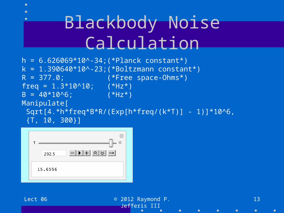
Blackbody Noise Calculation


h = 6.626069*10^-34;(*Planck constant*)k = 1.390640*10^-23;(*Boltzmann constant*)R = 377.0; (*Free space-Ohms*)freq = 1.3*10^10; (*Hz*)B = 40*10^6; (*Hz*)Manipulate[ Sqrt[4.*h*freq*B*R/(Exp[h*freq/(k*T)] - 1)]*10^6, {T, 10, 300}]


Thermal Noise - Microwave Frequencies

vRMS ≈ 4kTBR

At microwave frequencies the thermal noise is virtually independent of frequency, and the equation simplifies to:

vRMS = RMS voltage noise (Volts)

B = Bandwidth (Hz)R = Resistance (Ohms)k = Boltzmann constant

(1.3806404E-23 J/K)T = Temperature (Kelvin)

Goldstone Antenna


Wikipedia

This deep space radiotelescope system is outfitted with a cryogenically cooled receiver to lower the noise level for sensitive reception


Note

• The 500 kW CW X-band Goldstone Solar System RadarFreiley, A.; Quinn, R.; Tesarek, T.; Choate, D.; Rose, R.; Hills, D.; Petty, S.Microwave Symposium Digest, 1992., IEEE MTT-S InternationalVolume , Issue , 1-5 Jun 1992 Page(s):125 - 128 vol.1Digital Object Identifier ﾊ 10.1109/MWSYM.1992.187924Summary:In recent years the Goldstone Solar System Radar (GSSR) has undergone significant improvements in performance in the areas of increased transmitter power and increased receiver sensitivity. An overview of the radar system and each of these improvements are discussed. The transmitter was upgraded with two new state-of-the-art 250 kW X-band klystrons which increased the radiated power from 360 kW to 460 kW (1.1 dB). The microwave receiver system was improved by cryogenically cooling a major portion of the receive feed components, reducing the receiver noise temperature from 18.0 K to 14.7 K (0.9 dB).


Shot Noise

• Statistical noise due to the current carriers• The shot noise power in a resistor is,

P = 2qIBRwhere,q = electronic charge (1.602176E-19 Coul)I = average current [Amperes]B = Bandwidth [Hz]R = Resistance [Ohms]

• Shot noise arises in semi-conducting detectors


Flicker (1/f) Noise

• Usually found at low frequencies

• Can be ignored for microwaves


Solar Blackbody Radiation

• The sun is a HOT source (Blackbody temperature = 5778 K)(Microwave temperature = 136,000 K)

• Radiation is affected by sunspot cycles

• Radiation can cause significant interference at λ= 10.7 cm ( 1.07*108 nm ) or a frequency of ~28 GHz.


Solar Blackbody Radiation

The Columbus Optical SETI Observatory


Planck’s Radiation Law (ν,T)

where,I(ν,T) = Power Density (Watts · m-2 · ster-1 · Hz-1)h = Planck’s constant (6.62606896*10-34 J/s)c = velocity of light (2.99792458*108 m/s)ν= frequency (Hz)k = Boltzmann constant (1.3806504*10-23 J/K)T = temperature (e.g. 5778 K)

I(ν,T ) =2hν 3

c2

1e(hν /kT ) −1

⎛⎝⎜

⎞⎠⎟


Spectral Energy Density (ν,T)


Spectral Energy Density Calculation

h = 6.62606896*10^-34;k = 1.3806504*10^-23;T = 5778;c = 2.99792458*10^8;numin = 0.1*10^9;numax = 1000*10^9;Ilam = (2*h*nu^3/c^2)*(1/(Exp[(h*nu)/(k*T)] - 1));LogLogPlot[Ilam, {nu, numin, numax}, PlotStyle -> {Black, Thick}, Frame -> True, FrameLabel -> {"Frequency [GHz])", "Spectral Energy Density"}, LabelStyle -> Directive[Bold, Italic]]


Planck’s Radiation Law (λ,T)

I(λ,T ) =2 * 1024 hc2

λ5

1e(106 hc/λkT ) −1

⎛⎝⎜

⎞⎠⎟

where,I(n,T) = Power Density (Watts · m-2 · ster-1 · μm-1)h = Planck’s constant (6.62606896*10-34 J/s)c = velocity of light (2.99792458*108 m/s)λ= wavelength (μm)k = Boltzmann constant (1.3806504*10-23 J/K)T = temperature (e.g. 5778 K)


Spectral Energy Density (λ,T)


Solar Noise Power Density

N planck (ν,T ) =2πhν 3r2

c2R2

1e(hν /kT ) −1

⎛⎝⎜

⎞⎠⎟

where,N = Noise power density (Watts · m-2 · Hz-1)h = Planck’s constant (6.62606896*10-34 J/s)c = velocity of light (2.99792458*108 m/s)r = radius of Sun (6.955*108 m)ν= frequency (Hz)k = Boltzmann constant (1.3806504*10-23 J/K)T = temperature (Visible: 5778 K, Microwave: 27, 000)R = distance of receiver from Sun (1.49597870691*1011 m)


Solar Noise Spectral Energy Density


Solar Noise Spectral Energy Density

h = 6.62606896*10^-34;r = 6.955*10^8;k = 1.3806504*10^-23;R = 149597870691;T = 27000;c = 299792458;nu = c/(10^(lam/10));NN = (2*π*h*nu^3*r^2)/(c^2*(Exp[(h*nu)/(k*T)] -

1)*R^2);LogLogPlot[NN, {lam, 0.00000001, 1}, PlotStyle -> {Black, Thick}, Frame -> True, FrameLabel -> {"Wavelength [m])", "Spectral

Energy Density"}, LabelStyle -> Directive[Medium, Italic]]


Received Noise Power Formula

Pn = NPlanck(ν) · Ar

NPlanck = Noise Power Density integrated over bandwidth 36 MHz

= 6.26742*10-13 [Watts/m2]

Ar = Area of receiving antenna = 0.049 [m2] (Diam = 10λat 12 GHz)

B = Receiving input bandwidth [36 MHz]

Pn = 3.07226*10-14 [Watts] = -135.125 [dBW]


Received Noise Power Calculation

h = 6.62606896*10^-34;r = 6.955*10^8;k = 1.3806504*10^-23;R = 149597870691;T = 5778;c = 2.99792458*10^8;B = 36.0*10^6;numin = 12.0*10^9;numax = numin + B;lam0 = c/numin;ra = 10*lam0/2;Ar = π*ra^2NP = (2*π*h*nu^3*r^2)/(c^2*(Exp[(h*nu)/(k*T)] - 1)*R^2);NPD = NIntegrate[NP, {nu, numin, numax}]pn = NPD*Ar


Noise Model

• The Shannon - Weaver noise model treats noise as an additive effect on an otherwise noise-free communications channel for the purpose of calculating its effects


Noise Factors• The thermal noise calculated at the receiving antenna

output is:N0 = kTa [W/Hz]

• Input noise arises from a number of sources:– Blackbody temperature of space– Blackbody temperature of Sun– Atmospheric noise– Antenna blackbody noise– Receiver system noise calculated at the input

• These contributions can each be converted to equivalent noise temperatures

Noise Power

A black body at a temperature of T [Kelvins] generates electrical noise according to the relation,

where,

k = Boltzmann constant, 1.3806503*10-23 [J/K]

or -228.6 [dBW/K/Hz]

T = source temperature [Kelvins]

Bn = noise bandwidth [Hz]


Pn =kTBn

Boltzmann - Conversion to dBW


k = 1.3806503*10^-23;kdBW = 10*Log[10, k];Print["k [dBW] = ", kdBW]

k [dBW] = -228.599

Noise Power Conversion to dBm

• Noise power is frequently stated in dBm, or dB compared to 1 milliwatt.

• The dBm conversion for noise power is:


NdBm =10 logkTB0.001

⎡⎣⎢

⎤⎦⎥

Signal Power in Digital Transmission

• Carrier power is the average energy per bit, in a digital transmission

• Frequently stated in dBm• The conversion is:


CdBm =10 logCWatts

0.001⎡⎣⎢

⎤⎦⎥


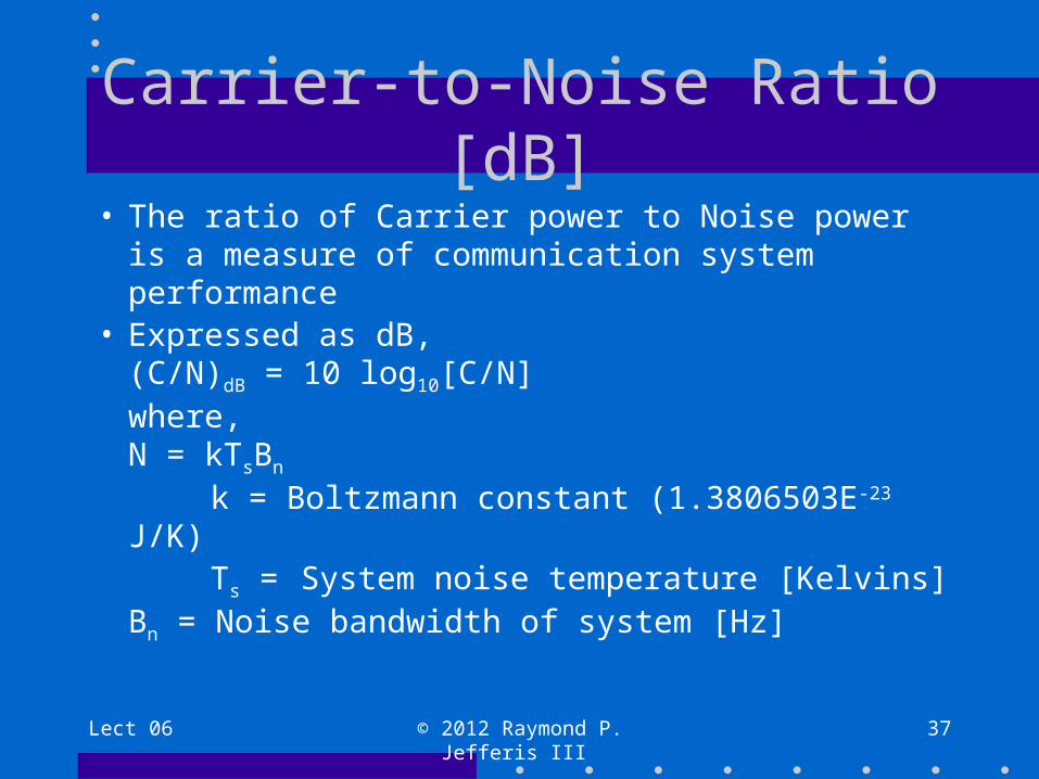
Carrier-to-Noise Ratio [dB]

• The ratio of Carrier power to Noise power is a measure of communication system performance

• Expressed as dB,(C/N)dB = 10 log10[C/N]where,N = kTsBn

k = Boltzmann constant (1.3806503E-23 J/K) Ts = System noise temperature [Kelvins]

Bn = Noise bandwidth of system [Hz]

Carrier-to-Noise Power Ratio

• Relates average carrier energy per bit, in digital transmission, to noise power density

• In dB (or dBm) units,


C

N⎛⎝⎜

⎞⎠⎟dB

=10 logCN

⎡⎣⎢

⎤⎦⎥=CdB −NdB

CN

⎛⎝⎜

⎞⎠⎟dBm

=10 logC / 0.001N / 0.001

⎡⎣⎢

⎤⎦⎥=CdBm −NdBm


C/N Ratio and Noise Temperature

Where,C = Carrier power [W]N = Noise power [W]

Pr = Received signal power

Pn = Received noise power

Ts = Equiv. input temp. [K]

Bn = Bandwidth of noise [Hz]

Tx = Equiv. temperature at x

Gx = Gain of stage x

k = Boltzmann constant (1.3806404E-23 J/K) or, -228.6

[dBW/HzK]

C

N=

Pr

Pn

where,attheinput,Pn =kTsBn

inwhich(tobediscussedlaterinmoredetail)Ts =Tin +TRF +TMix(1 / GRF ) +TIF (1 / GRFGMix)


Thermal Noise Power Model

The noise power Pn [Watts] delivered to the matched external resistor, R, is:

Pn =vRMS

2R⎛⎝⎜

⎞⎠⎟

2

R=kTB [Watts]

Energy per Bit

Where,Eb = energy per bit [Joules/bit]

fb = bit rate [bits/second]

Tb = time of bit [seconds]

C = Carrier power [Watts]

the energy per bit is:


Eb =C / fb =CTb

Noise Power Density

Where,N0 = noise power density [Watts/Hz]

N = thermal noise power [Watts]

B = Bandwidth [Hz]

the noise power density is:


N0 =NB

=kTBB

=kT

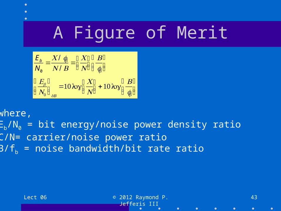
A Figure of Merit


Eb

N0

=C / fbN / B

=CN

⎛⎝⎜

⎞⎠⎟

Bfb

⎛

⎝⎜⎞

⎠⎟

Eb

N0

⎛

⎝⎜⎞

⎠⎟dB

=10 logCN

⎛⎝⎜

⎞⎠⎟+10 log

Bfb

⎛

⎝⎜⎞

⎠⎟

where,Eb/N0 = bit energy/noise power density ratioC/N= carrier/noise power ratioB/fb = noise bandwidth/bit rate ratio


Example: Earth Station Input

• C = 20 [Watts]

• B = 36*106 [Hz]

• T = 200 [K]

• k = 1.3806404*10-23 [J/K]

• Pn = (1.3806404*10-23)(200)(36*106) = 9.94*10-14 [Watts]

• CdBm = 10log[20/0.001] = 43.0103 [dBm]

• NdBm = 10log[9.94*10-14/0.001] = -100.026 [dBm]

• (C/N) dBm = CdBm – NdBm = 143.036 [dBm]


Example: Earth Station Input

• q = 1.602176E-19 [Coul]• I = 0.1E-3 [A] = 100 [μA]• B = 36E6 [Hz]• R = 50 [Ohms]• P = (2)(1.602176E-19 )(0.1E-3 )(36E6)(50) = 5.77*

10-14 [Watts]


Signal-to-Noise Ratio

• Ratio of signal power to noise powerSNR = Ps/Pn

• The dB form is frequently usedSNRdB = 10 log10(Ps/Pn)

• Is used as a performance measure


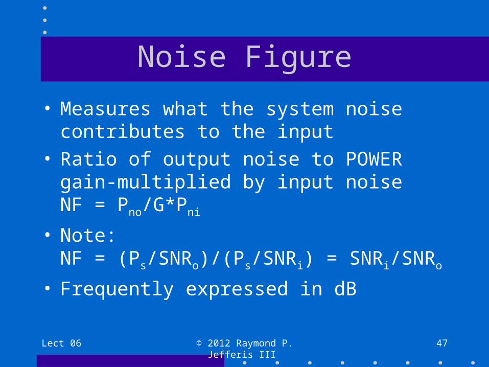
Noise Figure

• Measures what the system noise contributes to the input

• Ratio of output noise to POWER gain-multiplied by input noiseNF = Pno/G*Pni

• Note:NF = (Ps/SNRo)/(Ps/SNRi) = SNRi/SNRo

• Frequently expressed in dB


Noise Computations

• Noise Temperature (T) =290 * (10^(Noise Figure/10)-1) [K]

• Noise Figure (NF) =10 * log10 (Noise Factor) [dB]


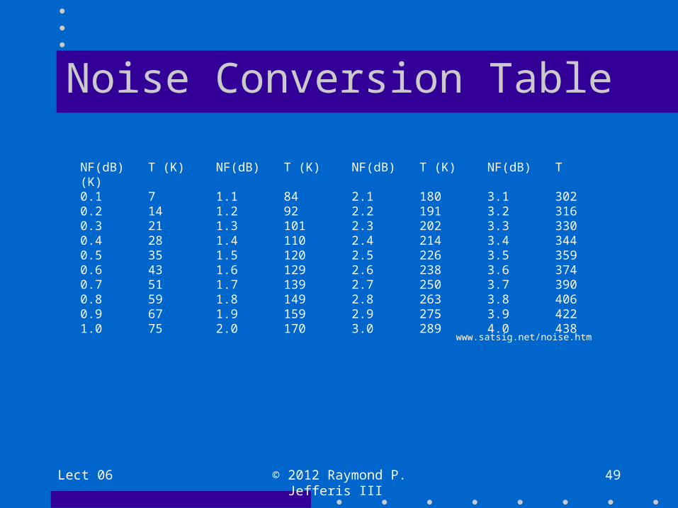
Noise Conversion Table

NF(dB) T (K) NF(dB) T (K) NF(dB) T (K) NF(dB) T (K)0.1 7 1.1 84 2.1 180 3.1 3020.2 14 1.2 92 2.2 191 3.2 3160.3 21 1.3 101 2.3 202 3.3 3300.4 28 1.4 110 2.4 214 3.4 3440.5 35 1.5 120 2.5 226 3.5 3590.6 43 1.6 129 2.6 238 3.6 3740.7 51 1.7 139 2.7 250 3.7 3900.8 59 1.8 149 2.8 263 3.8 4060.9 67 1.9 159 2.9 275 3.9 4221.0 75 2.0 170 3.0 289 4.0 438

www.satsig.net/noise.htm


Another Figure of Merit

• SPNN = (Ps + Pn) / Pn = 1+ SNR

• Channel Capacity (Shannon) as calculated using SPNNC = B log2(SPNN) [bits/sec]


Eb/N0 Ratio - Revisited

• Eb/N0 = (Signal energy per bit)/(Noise power density per Hertz)

Eb

N0

=PS / RN0

=PS

kTR

where,PS = Signal power [Watts = J/s]R = Data rate [bits/sec]τb = Time to send one bit = 1/R [sec]

Eb = Psτb = Energy per bit [J]T = Temperature [K]k = Boltzmann constant (1.3806404E-23 J/K)


Summary

Eb

N0

=PS / RN0

=PS

kTR=

PS

PN

⎛

⎝⎜⎞

⎠⎟BR

⎛⎝⎜

⎞⎠⎟

=SN

⎛⎝⎜

⎞⎠⎟

BR

⎛⎝⎜

⎞⎠⎟

N =N0B

References

• Stallings, W., Data and Computer Communications,Prentice-Hall, 2004.

• Tomasi, W., Advanced Electronic Communications Systems,Prentice-Hall, 2001.



Component Noise Model

Tn =Pn

kBPo = Pi + Pn( )Gn

To = Pi + Pn( )Gn

kB=

Pi

kB+

Pn

kB⎛⎝⎜

⎞⎠⎟Gn = Ti +Tn( )Gn


Meaning of Noise Model

• Noise temperatures can be treated additively

• The input noise plus the input-referred amplifier noise multiplied by the amplifier gain tields the effective noise temperature.


Noise Factor (Noise Figure)

• Another figure of merit for system components• Is defined at room temperature (290 K)• Noise balance

Output = G*(Input + Device)FGkT0 = Gk(T0+Td)The noise temperature of a device is:Td = (NF-1)T0

The noise figure of a device isNF = 1+ Td / T0


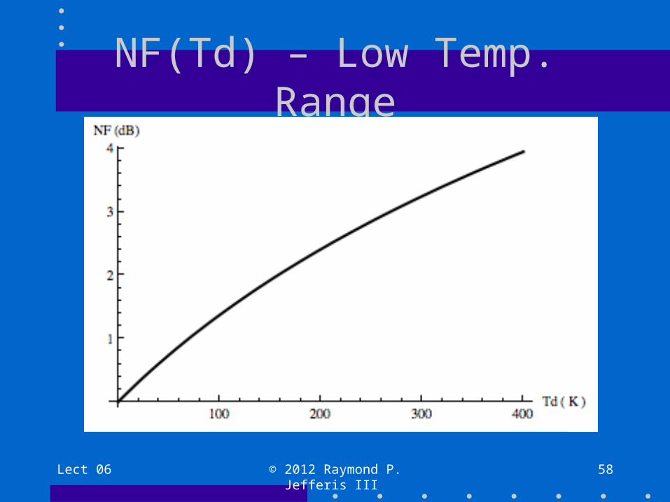
Noise Figure [dB]

• The noise figure of a device in dB is,NF = 10 log10[1+ Td / T0](See graph on next slide)

• T0 is typically assumed to be 290 K.


NF(Td) – Low Temp. Range


Noise Factor Calculation

T0 = 270;NF = 10 Log[10, 1 + Td/T0];Plot[NF, {Td, 0, 400},

AxesLabel -> {"Td ( K )", " NF (dB) "},

PlotStyle -> {Black, Thick}]


NFdB - Upper Temp. Range


Calculation of Noise Factor in dB

T0 = 270;NF = 10 Log[10, 1 + Td/T0];Plot[NF, {Td, 0, 10000},

AxesLabel -> {"Td ( K )", " NF (dB) "},

PlotStyle -> {Black, Thick}]


Cascaded System Components

Po2 =G2kTn2B+G1G2kB(Tn1 +Ti1)


Reference to Input TemperatureLet an input noise temperature, TS be defined. Then,

Po2 =G1G2kTSB

And thus,

Note that the first amplifier gain reducesthe noise temperature of the subsequent stage.

TS =(Tn1 +Ti1) +Tn2

G1


Noise Temperature Cascade Model

Pno3 =GIFkTIF B+GIFGmkTmB+GIFGmGRFkB(TRF +Tr )


Noise Temperature Model

Referring all noise to input,

TSource = Tr +TRF +Tm

GIF

+TIF

GmGRF

⎡

⎣⎢

⎤

⎦⎥


Carrier-to-Noise Ratio, C/N

• Similar to SNR, but more useful for FM transmission

C

N⎡⎣⎢

⎤⎦⎥dB

=[Pr ]dB −[Pn]dB

C

N⎡⎣⎢

⎤⎦⎥dB

= EIRP[ ]dB + Gr[ ]dB− LOSSi[ ]dB

− k[ ]dB − B[ ]dB − TS[ ]dBi∑

• Or, substituting the path loss results:


Typical Antenna Noise Temperatures

3.6m diameter antenna Model 8136 from ViaSat, C + Ku bands (Offset geometry)

Elevation angle (deg) Noise temp (C band) (K) Noise temp (Ku band) (K)10 24 3120 16 2330 15 2120 14 20

From www.satsig.net/antnoise.htm

4.7m diameter antenna Model Vertex, C + Ku bands

Elevation angle (deg) Noise temp (C band) (K) Noise temp (Ku band) (K)5 56 6910 40 6220 45 5740 42 52


Receiver Noise Figures

• Noise figures of 0.7 - 2.3 dB and gains of 22 - 27 dB can be achieved in Ku-band amplifiers.

• Noise Temperatures:– C-Band: 30 - 45 [K]

– Ku_Band: 75 - 85 [K]

• Si/Ge and Ga/As technologies are typically used• Cooling (thermoelectric, LN2, etc.) can reduce

noise temperatures


Amplifier Example: NEC NE32584

Noise Figure:NF = 0.45 dB Typ., Gain = 12.5 dB Typ. at f = 12 GHz

Application:C through Ku Band


Typical Component: NEC NE325501 Transistor

NF: 0.45 dB at 12 GHzGain: 12.5 dB at 12 GHz

From NE325501 Data sheet, NEC


End

Lect 06© 2012 Raymond P. Jefferis III1 Communications Noise Models The Shannon-Weaver noise model...

Documents

Transcript of Lect 06© 2012 Raymond P. Jefferis III1 Communications Noise Models The Shannon-Weaver noise model...