lec8 particle filter - courses.cs.washington.edu
59
1 Particle Filters Instructor: Chris Mavrogiannis TAs: Kay Ke, Gilwoo Lee, Matt Schmittle *Slides based on or adapted from Sanjiban Choudhury and Dieter Fox
Transcript of lec8 particle filter - courses.cs.washington.edu

1
Particle Filters
Instructor: Chris Mavrogiannis
TAs: Kay Ke, Gilwoo Lee, Matt Schmittle
*Slides based on or adapted from Sanjiban Choudhury and Dieter Fox

Assembling Bayes filter
2
TasksLocalization
P(pose | data)
Mapping P(map | data)
SLAM P(pose, map | data)
Belief Representations
Probabilistic Models
Bayes Filter

Tasks that we will cover
3
Tasks Belief Representation Probabilistic Models
Localization P(pose | data)
Gaussian / ParticlesMotion model
Measurement model
Mapping P(map | data)
Discrete (binary) Inverse measurement model
SLAM P(pose, map |
data)
Particles+Gaussian (pose, landmarks)
Motion model, measurement model, correspondence model
(Week 3)
(Week 4)
(Week 4)

Example: Indoor localization
4

Today’s objective
5
1. Understand the need for non-parametric filtering whenfaced with complex pdf in continuous space.
2. Importance sampling as an effective tool for dealing with complex pdf

Why can’t we just use parametric filters?
6
bel(xt) P (xt+1|zt+1)bel(xt+1)
(Gaussian)(Gaussian)(Gaussian)
bel(xt+1)
bel(xt) = ⌘P (zt|xt)
ZP (xt|xt�1, ut) bel(xt�1)dxt�1
(Gaussian)
Everything is a Gaussian - prior, motion, observation, posterior!

Good things about parametric filters
7
1. They are exact (when correct model)
E.g. Kalman Filter
2. They are efficient to compute
E.g. Sparse matrix inversion
We have so far been thinking about parametric filter (Kalman)
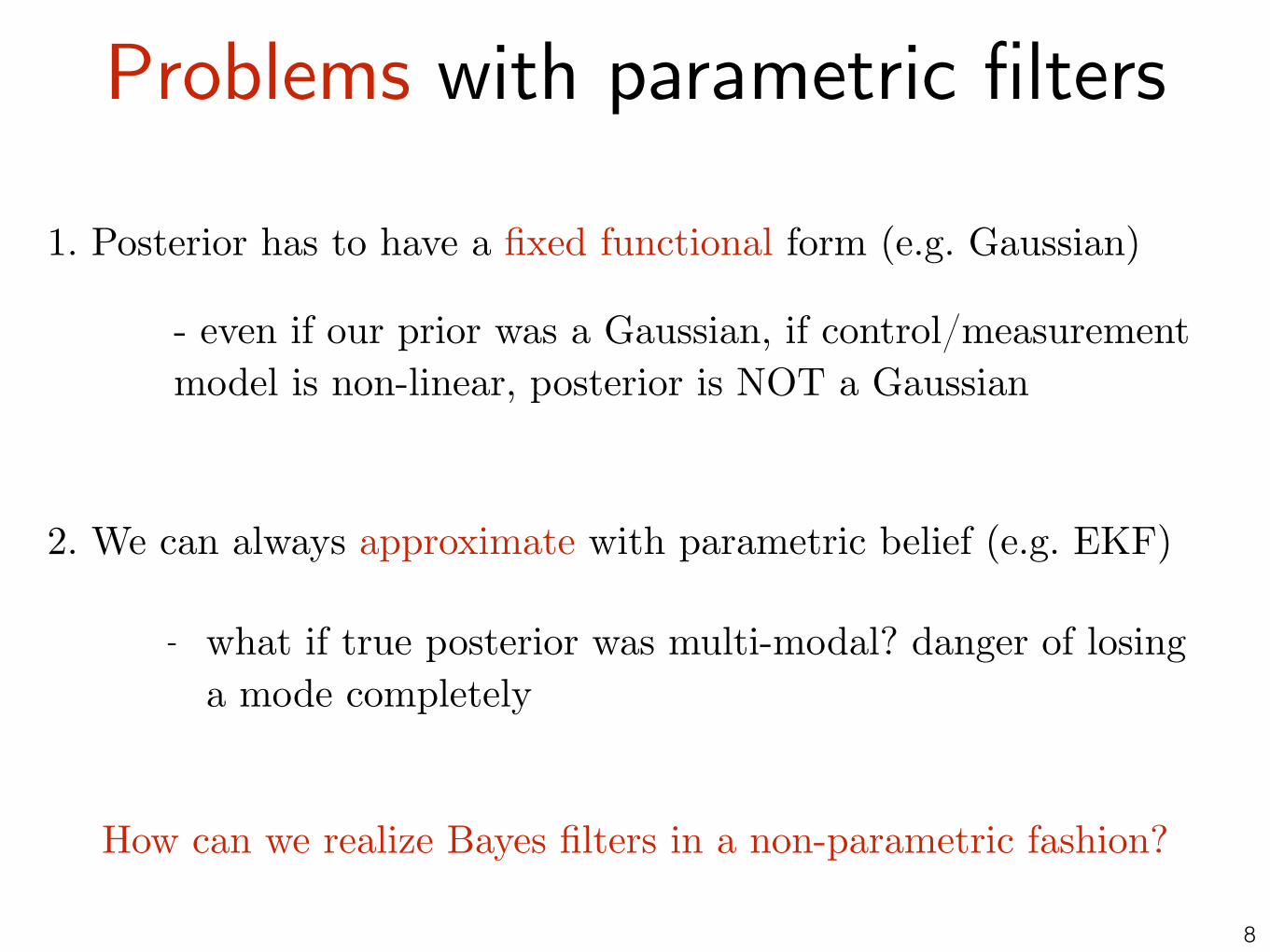
Problems with parametric filters
8
1. Posterior has to have a fixed functional form (e.g. Gaussian)
- even if our prior was a Gaussian, if control/measurementmodel is non-linear, posterior is NOT a Gaussian
2. We can always approximate with parametric belief (e.g. EKF)
- what if true posterior was multi-modal? danger of losinga mode completely
How can we realize Bayes filters in a non-parametric fashion?

Tracking a landing pad with laser only
9(Arora et al.)

10
Question: What are our options for non-parametric
belief representations?
1. Histogram filter
2. Normalized importance sampling
3. Particle filter
Approach 1: Histogram filter
11
Simplest approach - discretize the space!
Prior Posteriorbel(xt) bel(xt+1)

Example: Grid-based localization
12

Issues with grid-based localization
13
1. Curse of dimensionality
2. Wasted computational effort
3. Wasted memory resources
Remedy: Adaptive discretization
Remedy: Pre-cache measurements from cell centers
Remedy: Update a select number of cells only

14
If discretization is expensive, can we sample?

Monte-Carlo method
15
Q: What do we intend to do with the belief ? bel(xt+1)
Ans: Often times we will be evaluating the expected value
E[f ] =Z
xf(x)bel(x)dx
Mean position:
Probability of collision:
Mean value / cost-to-go:
f(x) ⌘ x
f(x) ⌘ I(x 2 O)
f(x) ⌘ V (x)

Monte-Carlo method
16
E[f ] =Z
xf(x)bel(x)dx
Problem: Can’t evaluate the integral below since we don’t know bel
E[f ] ⇡ 1
N
NX
i
f(xi)
Solution: Sample from the distribution
(originated in Los Alamos)
+ Incremental, any-time.
+ Converges to the true expectation under a mild set of assumptions
Lots of general applications!
x1, . . . , xN ⇠ bel(x)
Monte Carlo Estimate

Can we always sample?
17
bel(xt) = ⌘P (zt|xt)
Zp(xt|ut, xt�1)bel(xt�1)dxt�1
How can we sample from the product of two distributions?

18
Question: How can we sample from a complex distribution p(x)?

Solution: Importance sampling
19
Trick: 1. Sample from a proposal distribution (easy), 2. Reweigh samples to fix it!

Solution: Importance sampling
20
Don’t know how to generate these samples!!
p(x)
Target

Solution: Importance sampling
21
Trick: 1. Sample from a proposal distribution (easy),
p(x) q(x)
ProposalTarget

Solution: Importance sampling
22
Trick: 1. Sample from a proposal distribution (easy), 2. Reweigh samples to fix it!
p(x) q(x)
ProposalTarget

Convergence precondition:
Solution: Importance sampling
23
Trick: Sample from a proposal distribution (easy), reweigh samples to fix it!
Ep(x)
[f(x)] =X
p(x)f(x) (1a)
=X
p(x)f(x)q(x)
q(x)(1b)
=X
q(x)p(x)
q(x)f(x) (1c)
= Eq(x)
[p(x)
q(x)f(x)] (1d)
⇡ 1
N
NX
i=1
p(xi)
q(xi)f(xi). (1e)
p(x)q(x) is called the importance weight. When we are undersampling an area, it weights it stronger;likewise, oversampled areas are weighted more weakly.
Consider the following (somewhat contrived) pair of functions:
Figure 2: Comparison of distribution we wish to sample from, p, and distribution we can samplefrom, q.
Notice that there are places where p is nonzero and q is zero, which means we have regions tosample that we aren’t sampling at all.
Our estimate of the expectation of p becomes:
1
N
NX
i=1
p(xi)
q(xi)f(xi) !N!1 Ep[f(x)] (2)
2.1 Example
Set q as the motion model. Note that in reality we never use this – we use a better approximationof p(xt|xt�1) because the motion model takes too many samples to be reliable.
2
p(x) > 0 q(x) > 0whenever
Importance Weight

Question: What makes a good proposal distribution?
24
p(x) q(x)

25
bel(xt) = ⌘P (zt|xt)
Zp(xt|ut, xt�1)bel(xt�1)dxt�1
Target distribution : Posterior
Proposal distribution : After applying motion model
bel(xt) =
Zp(xt|ut, xt�1)bel(xt�1)dxt�1
Applying importance sampling to Bayes filtering
Importance ratio:
r =bel(xt)
bel(xt)= ⌘P (zt|xt)w

26
Question: What are our options for non-parametric
belief representations?
1. Histogram filter
2. Normalized importance sampling
3. Particle filter

Approach 2: Normalized Importance Sampling
27
bel(xt�1) =
⇢x1t�1
w1t�1
,x2t�1
w2t�1
, · · · , xMt�1
wMt�1
�0.5
0.25
0.25
for i = 1 to M
sample xit ⇠ P (xt|ut, x
it)
0.5
0.25
0.25
0.5 * 0.02
0.25 * 0.1
0.25 * 0.05
for i = 1 to M
wit = P (zt|xi
t)wit�1
=0.01
=0.025
=0.0125
for i = 1 to M
wit =
witP
i wit
0.21
0.53
0.26bel(xt) =
⇢x1t
w1t, · · · , x
Mt
wMt
�

Problem: What happens after enough iterations?
28
Particles don’t move - can get stuck in regions of low probability
This is a problem of histogram filters too…
True posterior True posterior True posterior
29
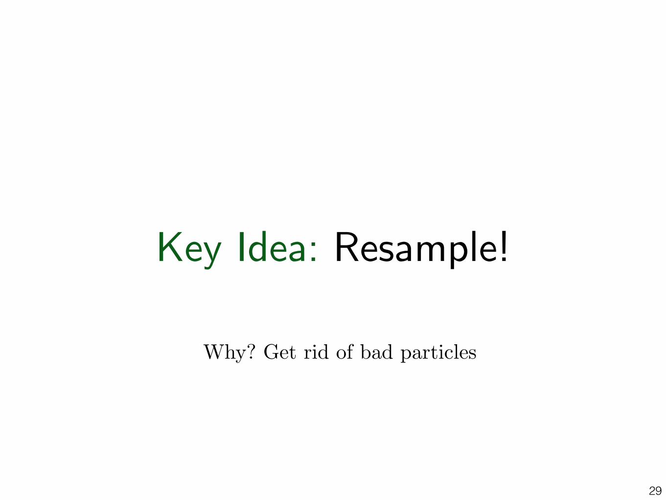
Key Idea: Resample!
Why? Get rid of bad particles

Approach 3: Particle Filtering (with IS)
30
for i = 1 to M
sample xit ⇠ P (xt|ut, x
it)
for i = 1 to Mfor i = 1 to M
for i = 1 to M
bel(xt�1) =
⇢x1t�1
w1t�1
,x2t�1
w2t�1
, · · · , xMt�1
wMt�1
�0.5
0.25
0.25
0.5
0.25
0.25
0.5 * 0.02
0.25 * 0.1
0.25 * 0.05
=0.01
=0.025
=0.0125
all weights = 1/M
wit = P (zt|xi
t)wit�1
for i = 1 to M
sample xit ⇠ wi
tbel(xt) =
⇢x1t
1, · · · , x
Mt
1
�2

Virtues of resampling
31
ut zt ut+1 zt+1resample
2
resample
3

Why use particle filters?
32
1. Can answer any query
2. Will work for any distribution, including multi-modal (unlike Kalman filter)
3. Scale well in computational resources (embarrassingly parallel)
4. Easy to implement!

33

34

35

36

37

38

39

40

41
Histogram Filter
Normalized Importance Sampling
Particle Filter
Grid up state space
Use a fixed set of samples
Resample
Non-parametric FiltersSa
me
fund
amen
tal B
ayes
rul
e ag
ain
and
agai
n …

42
Are we done?
No! Lots of practical
problems to deal with

Problem 1: Two room challenge
43
(a) Two rooms with equal probability (b) The same filter, after repeated resampling
Figure 4: A problem with assuming the independence of the observations and using naıve sampling.Without gaining any new information, the particle filter converges on one of the rooms.
the same observations; however, over the course of 100 timesteps, the filter has become certain thatit is in the right room.
What has happened? The filter is non-deterministic, and so when we pick the particles withequal weight, it is unlikely that we will equal numbers from each room. As time progresses, thisselection process only becomes more imbalanced: with observations equally likely, if a state has veryfew particles in its vicinity, in expection, it will have very few particles after resampling. Further,once a state space loses its particles, there are no ways to regain them without motion happening.
Figure 5: Low Variance Resampling; in practice, this approach is preferred over the naıve approach.
Fixes: There are a number of ways to prevent situations like this from happening in practice.
1. One way is to detect situations in which you do not have enough new information to resam-ple, and only run the resampling when your observation model has su�ciently new obser-vation data to process. One statistic that might be useful for evaluting this is looking atmax({wi})/min({wi}), or looking at the entropy of the weights.
2. One easy fix is to run a more sophisticated resampling method, the low-variance resampler. Inthis approach, which is depicted in Fig. 5, a single number r is drawn, and then particles areselected at every 1/N units on the dartboard in our example. E↵ectively, the same sampler isused, but the random numbers generated are r+i/N for all (positive and negative) i such thatr + i/N 2 [0, 1]. This has desirable properties: for instance, every particle with normalizedweight over 1/N is guaranteed to be selected at least once. Due to these properties and itsease of implementation, it is always recommended that you implement this sampler ratherthan the naıve approach. Note that this is also known as the “Stochastic Universal Sampler”,in the genetic algorithms domain.
3. One easy, but undesirable approach is to just inject uniform samples. This should be treatedas a last resort as it is unprincipled.
5
Given: Particles equally distributed, no motion, no observation
What happens?
All particles migrate to the other room!!
(a) Two rooms with equal probability (b) The same filter, after repeated resampling
Figure 4: A problem with assuming the independence of the observations and using naıve sampling.Without gaining any new information, the particle filter converges on one of the rooms.
the same observations; however, over the course of 100 timesteps, the filter has become certain thatit is in the right room.
What has happened? The filter is non-deterministic, and so when we pick the particles withequal weight, it is unlikely that we will equal numbers from each room. As time progresses, thisselection process only becomes more imbalanced: with observations equally likely, if a state has veryfew particles in its vicinity, in expection, it will have very few particles after resampling. Further,once a state space loses its particles, there are no ways to regain them without motion happening.
Figure 5: Low Variance Resampling; in practice, this approach is preferred over the naıve approach.
Fixes: There are a number of ways to prevent situations like this from happening in practice.
1. One way is to detect situations in which you do not have enough new information to resam-ple, and only run the resampling when your observation model has su�ciently new obser-vation data to process. One statistic that might be useful for evaluting this is looking atmax({wi})/min({wi}), or looking at the entropy of the weights.
2. One easy fix is to run a more sophisticated resampling method, the low-variance resampler. Inthis approach, which is depicted in Fig. 5, a single number r is drawn, and then particles areselected at every 1/N units on the dartboard in our example. E↵ectively, the same sampler isused, but the random numbers generated are r+i/N for all (positive and negative) i such thatr + i/N 2 [0, 1]. This has desirable properties: for instance, every particle with normalizedweight over 1/N is guaranteed to be selected at least once. Due to these properties and itsease of implementation, it is always recommended that you implement this sampler ratherthan the naıve approach. Note that this is also known as the “Stochastic Universal Sampler”,in the genetic algorithms domain.
3. One easy, but undesirable approach is to just inject uniform samples. This should be treatedas a last resort as it is unprincipled.
5

Reason: Resampling increases variance
44
Resampling collapses particles, reduces diversity, increases variance w.r.t true posterior
Particles
True posteriorresample resample

Fix 1: Choose when to resample
45
Key idea: If variance of weights low, don’t resample
We can implement this condition in various ways
1. All weights are equal - don’t resample
2. Entropy of weights high - don’t resample
3. Ratio of max to min weights low - don’t resample

Fix 2: Low variance sampling
46
4
w2
w3
w1wn
Wn-1
Resampling
w2
w3
w1wn
Wn-1
• Roulette wheel• Binary search, n log n
• Stochastic universal sampling• Systematic resampling• Linear time complexity• Easy to implement, low variance
1. Algorithm systematic_resampling(S,n):
2.3. For Generate cdf4.5. Initialize threshold
6. For Draw samples …7. While ( ) Skip until next threshold reached8.9. Insert10. Increment threshold
11. Return S�
Resampling Algorithm
11,' wcS =Æ=
ni !2=i
ii wcc += -1
1],,0[~ 11 =- inUu
nj !1=
1-+= nuu jj
ij cu >
{ }><È= -1,'' nxSS i
1+= ii
Also called stochastic universal sampling
Particle Filters)|(
)()()|()()|()(
xzpxBel
xBelxzpw
xBelxzpxBel
aaa
=¬
¬
-
-
-
Sensor Information: Importance Sampling

Fix 2: Low variance sampling
47
4
w2
w3
w1wn
Wn-1
Resampling
w2
w3
w1wn
Wn-1
• Roulette wheel• Binary search, n log n
• Stochastic universal sampling• Systematic resampling• Linear time complexity• Easy to implement, low variance
1. Algorithm systematic_resampling(S,n):
2.3. For Generate cdf4.5. Initialize threshold
6. For Draw samples …7. While ( ) Skip until next threshold reached8.9. Insert10. Increment threshold
11. Return S�
Resampling Algorithm
11,' wcS =Æ=
ni !2=i
ii wcc += -1
1],,0[~ 11 =- inUu
nj !1=
1-+= nuu jj
ij cu >
{ }><È= -1,'' nxSS i
1+= ii
Also called stochastic universal sampling
Particle Filters)|(
)()()|()()|()(
xzpxBel
xBelxzpw
xBelxzpxBel
aaa
=¬
¬
-
-
-
Sensor Information: Importance Sampling
Assumption: weights sum to 1

Why does this work?
48
4
w2
w3
w1wn
Wn-1
Resampling
w2
w3
w1wn
Wn-1
• Roulette wheel• Binary search, n log n
• Stochastic universal sampling• Systematic resampling• Linear time complexity• Easy to implement, low variance
1. Algorithm systematic_resampling(S,n):
2.3. For Generate cdf4.5. Initialize threshold
6. For Draw samples …7. While ( ) Skip until next threshold reached8.9. Insert10. Increment threshold
11. Return S�
Resampling Algorithm
11,' wcS =Æ=
ni !2=i
ii wcc += -1
1],,0[~ 11 =- inUu
nj !1=
1-+= nuu jj
ij cu >
{ }><È= -1,'' nxSS i
1+= ii
Also called stochastic universal sampling
Particle Filters)|(
)()()|()()|()(
xzpxBel
xBelxzpw
xBelxzpxBel
aaa
=¬
¬
-
-
-
Sensor Information: Importance Sampling
1. What happens when all weights equal?
2. What happens if you have ONE large weight and many tiny weights?
w1 = 0.5, w2 = 0.5/1000, w3 = 0.5/1000, …. w1001 = 0.5/1000

Problem 2: Particle Starvation
49
No particles in the vicinity of the current state
Why?1. Unlucky set of samples
2. Committed to the wrong mode in a multi-modal scenario 3. Bad set of measurements

Fix: Add new particles
50
Which distribution should be used to add new particles?
1. Uniform distribution
2. Biased around last good measurement
3. Directly from the sensor model

Fix: Add new particles
51
When should we add new samples?
Key Idea: As soon as importance weights become too small, add more samples
1. Threshold the total sum of weights
2. Fancy estimator that checks rate of change.

Problem 3: Observation model too good!
52
Observation model is so peaky, that all particles die!
1. Sample from a better proposal distribution than motion model!
2. Squash the observation model (apply a power of 1/m to all probabilities. m observations count as one)
3. Last resort: Smooth your observation model with a Gaussian (you are pretending your observation model is worse than it is)
Fixes

Fix 1: Sample from a better proposal distribution
53
Key Idea: Sample and weigh particles correctly
Contact observation may kill ALL particles!
bel(xt) = ⌘P (zt|xt)
ZP (xt|xt�1, ut) bel(xt�1)dxt�1
(Sample) (Reweigh)
Koval et al. 2017

Problem 4: How many samples is enough?
54
Example: We typically need more particles at the beginning of run
Key idea: KLD Sampling (Fox et al. 2002)
1. Partition the state-space into bins
2. When sampling, keep track of the number of bins
3. Stop sampling when you reach a statistical threshold that depends on the number of bins
(If all samples fall in a small number of bins -> lower threshold)

Page 14!
KLD-sampling
KLD-sampling
55
KLD sampling

Closing: Myth busting Particle filters
56
1. Particle Filter = Sample from motion model, weight by observation
(sample from any good proposal distribution)
2. Particle filters are for localization
3. Particle filters are to do with samples
(any continuous space estimation problem)
(normalized importance sampling also uses samples but no resampling)

57
Estimate state
Control robot to
follow plan
Plan a sequence of
motions

58
Bayes filter in a nutshell
bel(xt)
zt
ut
bel(xt)
Step 1: Prediction - push belief through dynamics given action
bel(xt) =
ZP (xt|ut, xt�1)bel(xt�1)dxt�1
Step 2: Correction - apply Bayes rule given measurement
bel(xt) = ⌘P (zt|xt)bel(xt)
bel(xt�1)

Bayes filter is a powerful tool
59Localization Mapping SLAM POMDP