LEBESGUE MEASURE THEORETIC DYNAMICS OFRATIONAL MAPS

JANE HAWKINS

Abstract. We survey the role of one and two dimensional Lebesguemeasure in complex dynamics. Before computers, rational mapswith Julia set the whole sphere, a circle, or an arc were the onlyaccessible maps so we begin with these classical examples. Wethen discuss some more recently studied families of rational mapsthat preserve finite or infinite measures equivalent to one and twodimensional Lebesgue measure. We end with a brief look at theidea behind Julia sets of quadratic polynomials with positive two-dimensional Lebesgue measure.

1. Introduction

Ever since the advent of computers, interest in the measurable dy-namics of rational maps whose Julia sets are either the sphere or asmooth arc has been overshadowed by the multitude of beautifully illus-trated studies of measures supported on fractal Julia sets. The fractalmeasures considered are a natural generalization of Lebesgue measureto noninteger dimension. However Lebesgue measurable dynamics stillplay an important and interesting role in the field of complex dynam-ics. One of the deepest results in the field in the past decade was theconstruction and proof of a Julia set which has positive area, but is notthe entire sphere [12].

In this short survey article we start with the classical examples andmove to more unusual families of rational maps of the Riemann spherethat exhibit interesting Lebesgue measurable dynamics. Many of theresults mentioned in this paper have appeared elsewhere but we bringthem together here under this common theme of Lebesgue measurabledynamics of rational maps. One of the main points of this survey is toillustrate that in the midst of fractal Julia sets lie many parametrizedfamilies of maps with smooth Julia sets and chaotic Lebesgue measuretheoretic behavior.

In Section 2 we lay some groundwork with basic definitions and theclassical examples. We continue the discussion in this section with two

Date: March 25, 2016.1

2 JANE HAWKINS

families of maps with chaotic one dimensional behavior; the measurewe use is the arc length measure of a one-dimensional subset on thesphere, which we denote by m1. One family of maps has the propertythat it is a nonpolynomial family (except for one map) of S-unimodalmaps all of which are ergodic, exact, and admit an equivalent invariantprobably measure.

The next family is parametrized by one real parameter, and eachmap preserves Lebesgue measure ` on R, the Julia set of each map.We connect these maps to inner functions by showing they are squareroots of them. Many of the results in this section were obtained by twoof the author’s Ph.D. students [6, 17].

We then turn to m2, normalized surface area measure in Section 4;we begin with a quick view of the Lattes examples dating back to 1918and we then move forward to the 1980s and look at postcritically finiterational maps more generally. Theorem 4.1 is a new result. In Section4.4 we give a brief idea of how one can show a Julia set for a polynomialcould have positive m2 measure.

The author thanks the co-organizers and hosts at Bryn Mawr andWilliams College for the Oxtoby Centennial Conferences. Work of Ox-toby inspired this measurable approach to complex dynamics. Theauthor is also grateful to the referee for suggestions that greatly im-proved the exposition in this paper.

2. Preliminary definitions and the first examples

We start with the first two classical examples of rational maps thatone studies; they have smooth Julia sets. They are p0(z) = z

2 andthe polynomial occurring at the tip of the Mandelbrot set: p�2(z) =z

2 � 2. The second map is more often presented to us as the degreetwo Chebychev polynomial ⌧2(z) = 2z2 � 1. The maps p�2 and ⌧2 arerelated via the map �(z) = 2z, which maps [�1, 1] linearly onto [�2, 2],and satisfies � � ⌧2(z) = p�2 � �(z).

Throughout this paper we let C1 denote the Riemann sphere. The

maps of interest are rational maps of the form: R(z) =p(z)

q(z), with

p, q polynomials over C with no common factor, and such that themaximum degree of p and q is at least 2. Rational maps characterizethe analytic maps of the Riemann sphere; by R

n we denote the n-foldcomposition of R with itself. Two rational maps R, S : C1 ! C1 areconformally conjugate if there exists a linear fractional transformation� on C1 such that

(1) � �R = S � �.

LEBESGUE DYNAMICS 3

We showed above that p�2 and ⌧2 are conformally conjugate maps.The notion of conjugacy has a few meanings in this setting. It often

occurs that we have two rational maps R, S related by a map � on C1such that � �R = S ��, but � is only continuous, in which case we sayR and S are topologically conjugate.

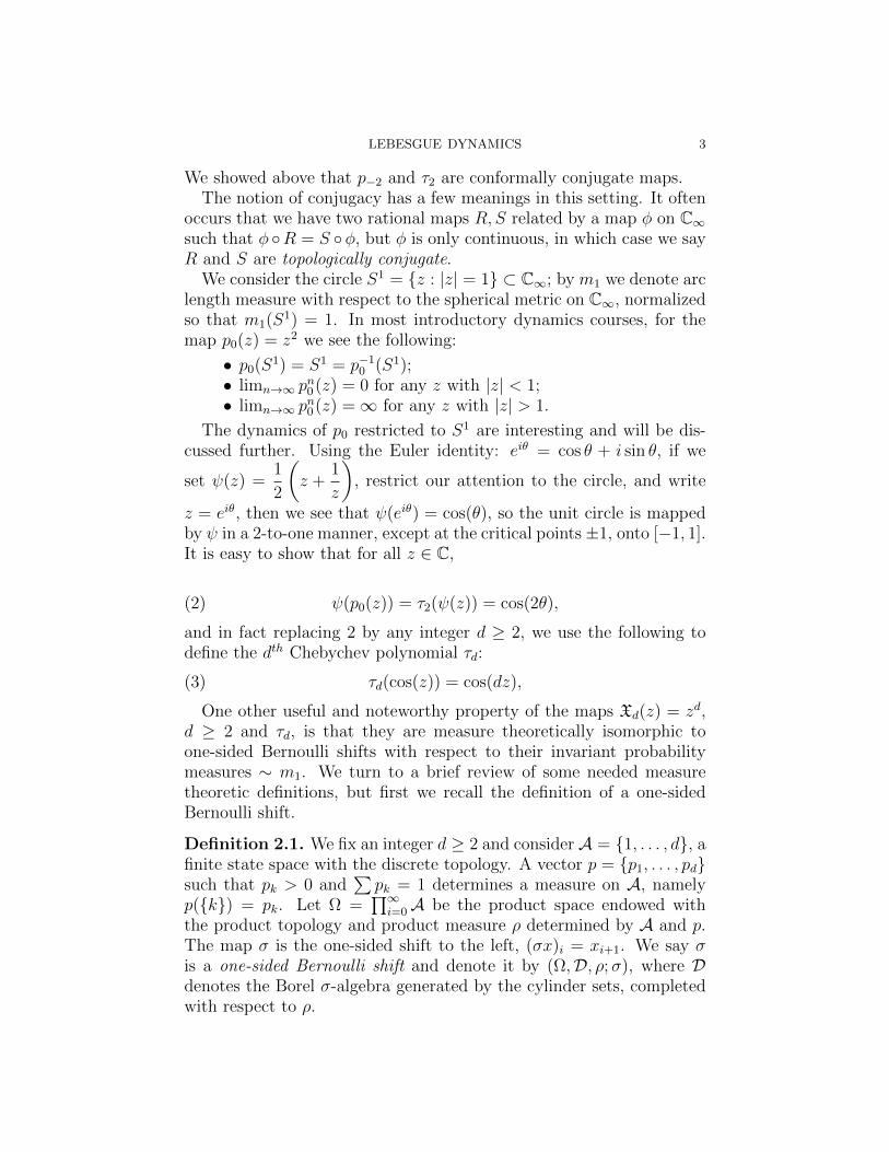
We consider the circle S1 = {z : |z| = 1} ⇢ C1; by m1 we denote arclength measure with respect to the spherical metric on C1, normalizedso that m1(S1) = 1. In most introductory dynamics courses, for themap p0(z) = z

2 we see the following:

• p0(S1) = S

1 = p

�10 (S1);

• limn!1 p

n

0 (z) = 0 for any z with |z| < 1;• lim

n!1 p

n

0 (z) = 1 for any z with |z| > 1.

The dynamics of p0 restricted to S

1 are interesting and will be dis-cussed further. Using the Euler identity: e

i✓ = cos ✓ + i sin ✓, if we

set (z) =1

2

✓z +

1

z

◆, restrict our attention to the circle, and write

z = e

i✓, then we see that (ei✓) = cos(✓), so the unit circle is mappedby in a 2-to-one manner, except at the critical points±1, onto [�1, 1].It is easy to show that for all z 2 C,

(2) (p0(z)) = ⌧2( (z)) = cos(2✓),

and in fact replacing 2 by any integer d � 2, we use the following todefine the d

th Chebychev polynomial ⌧d

:

(3) ⌧

d

(cos(z)) = cos(dz),

One other useful and noteworthy property of the maps Xd

(z) = z

d,d � 2 and ⌧

d

, is that they are measure theoretically isomorphic toone-sided Bernoulli shifts with respect to their invariant probabilitymeasures ⇠ m1. We turn to a brief review of some needed measuretheoretic definitions, but first we recall the definition of a one-sidedBernoulli shift.

Definition 2.1. We fix an integer d � 2 and consider A = {1, . . . , d}, afinite state space with the discrete topology. A vector p = {p1, . . . , pd}such that p

k

> 0 andP

p

k

= 1 determines a measure on A, namelyp({k}) = p

k

. Let ⌦ =Q1

i=0 A be the product space endowed withthe product topology and product measure ⇢ determined by A and p.The map � is the one-sided shift to the left, (�x)

i

= x

i+1. We say �is a one-sided Bernoulli shift and denote it by (⌦,D, ⇢; �), where Ddenotes the Borel �-algebra generated by the cylinder sets, completedwith respect to ⇢.

4 JANE HAWKINS

2.1. Measure theoretic preliminaries. We assume throughout thatevery space (X,B, µ) under consideration is a Lebesgue probabilityspace though sometimes we specify that µ is a �-finite infinite measure.In our setting, X ⇢ C1 is always a closed set and B denotes the �-algebra of Borel measurable sets. We assume that the measure spaceis complete with respect to µ (every subset of every null set for µ ismeasurable), and that T is a surjective nonsingular endomorphism;i.e., T : X ! X satisfies: µ(A) = 0 () µ(T�1

A) = 0 for everyA 2 B, and µ(T (X)4X) = 0. If ⌫ is a �-finite measure such that⌫ ⇠ µ, and ⌫(T�1

A) = ⌫(A) for all A 2 B, we say that T is measure-

preserving, or equivalently T preserves ⌫. Without loss of generality wecan assume that T is forward measurable and forward nonsingular; i.e.,for all measurable sets A, T (A) 2 B and µ(A) = 0 () µ(TA) = 0.When we say that a property holds on X (µ mod 0) or µ a.e., we meanthat there is a set N 2 B with µ(N) = 0, (N is possibly the emptyset), such that the property holds for all x 2 X \N .

Definition 2.2. Let T1 : (X1,B1, µ1) and T2 : (X2,B2, µ2) be twomeasure-preserving endomorphisms.

A measurable map � : X1 ! X2 is a homomorphism if there existsa set Y1 2 B1 of full measure and a set Y2 2 B2 of full measure in X2

such that � maps Y1 onto Y2.If there exists a homomorphism � such that T1(Y1) = Y1, T2(Y2) =

Y2, � � T1 = T2 � � on Y1, and µ2(A) = µ1(��1(A)) for all A 2 B1, thenT2 is called a factor of T1 (w.r.t. the measures µ1 and µ2), with factor

map �.If in addition � is injective on Y1 we say it is an isomorphism. If

T2 is a factor of T1 and � is an isomorphism, then we say that theendomorphisms T1 and T2 are isomorphic endomorphisms.

For any two sets A,B 2 B we define A4B = (A \B)[ (B \A). Themap T is ergodic if T has a trivial field of invariant sets, or equivalently,if any measurable set T with the property that µ(B4T

�1B) = 0 has

either zero or full measure.A map is exact if it has a trivial tail field \

n�0T�nB ⇢ B, or equiv-

alently, if any set B with the property µ(T�n � T n(B)4B) = 0 for alln has either zero or full measure. It is clear that every exact map isalso ergodic.

Assume T : (X,B, µ) ! (X,B, µ) preserves µ. We recall a conditionwhich is strictly weaker than one-sided Bernoulli for endomorphisms[16], but equivalent to Bernoulli in the invertible case [15]. We referthe reader to [11, 23, 24] if more detail is needed.

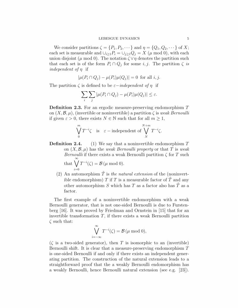
LEBESGUE DYNAMICS 5

We consider partitions ⇣ = {P1, P2, · · · } and ⌘ = {Q1, Q2, · · · } of X;each set is measurable and [

i�1Pi

= [j�1Qj

= X (µ mod 0), with eachunion disjoint (µ mod 0). The notation ⇣_⌘ denotes the partition suchthat each set is of the form P

i

\ Q

j

for some i, j. The partition ⇣ is

independent of ⌘ if

|µ(Pi

\Q

j

)� µ(Pi

)µ(Qj

)| = 0 for all i, j.

The partition ⇣ is defined to be "�independent of ⌘ ifX

i

X

j

|µ(Pi

\Q

j

)� µ(Pi

)µ(Qj

)| ".

Definition 2.3. For an ergodic measure-preserving endomorphism T

on (X,B, µ), (invertible or noninvertible) a partition ⇣ is weak Bernoulliif given " > 0, there exists N 2 N such that for all m � 1,

m_

0

T

�i

⇣ is "� independent ofN+m_

N

T

�i

⇣.

Definition 2.4. (1) We say that a noninvertible endomorphism T

on (X,B, µ) has the weak Bernoulli property or that T is weakBernoulli if there exists a weak Bernoulli partition ⇣ for T such

that1_

i=0

T

�i(⇣) = B (µ mod 0).

(2) An automorphism T is the natural extension of the (noninvert-ible endomorphism) T if T is a measurable factor of T and anyother automorphism S which has T as a factor also has T as afactor.

The first example of a noninvertible endomorphism with a weakBernoulli generator, that is not one-sided Bernoulli is due to Fursten-berg [16]. It was proved by Friedman and Ornstein in [15] that for aninvertible transformation T , if there exists a weak Bernoulli partition⇣ such that:

1_

i=�1

T

�i(⇣) = B (µ mod 0),

(⇣ is a two-sided generator), then T is isomorphic to an (invertible)Bernoulli shift. It is clear that a measure-preserving endomorphism T

is one-sided Bernoulli if and only if there exists an independent gener-ating partition. The construction of the natural extension leads to astraightforward proof that the a weakly Bernoulli endomorphism hasa weakly Bernoulli, hence Bernoulli natural extension (see e.g. [23]).

6 JANE HAWKINS

Weakly Bernoulli endomorphisms exhibit many highly mixing prop-erties, and conditions under which piecewise smooth bounded-to-oneinterval maps are weakly Bernoulli were given by Ledrappier in [23].

When we endow the Riemann sphere C1 with the �-algebra of Borelsets, we consider rational maps R and nonsingular Borel measures µ

for R, supported on the Julia set J(R) (see Defn 3.1) , such that R is anonsingular d-to-1 endomorphism of C1, where d is the degree of themap. We only consider measures with respect to which R is d-to-onein the following measurable sense.

Definition 2.5. A nonsingular map T on (X,B) is d-to-one with re-spect to a measure µ if there exists a partition ⇣ = {A1, A2, . . . Ad

} ofX into d disjoint atoms of positive measure, called a Rohlin partition,and satisfying:

(1) the restriction of T to each A

i

, which we will write as T

i

, isone-to-one (µ mod 0);

(2) each A

i

is of maximal measure in X \ [j<i

A

j

with respect toproperty (1);

(3) T

i

is one-to-one and onto X (µ mod 0) for i = 1, . . . , d.

3. A family of ergodic and exact nonpolynomial mapswith an invariant probability measure equivalent to `

The stereographic projection map S takes C1\{1} injectively ontoC, and circles containing {1} and their arcs are mapped to lines andline segments under S. Moreover on these sets the measure S⇤m1 ⇠ `,therefore when we consider rational maps in C we use Lebesgue mea-sure ` on R if the Julia set is a line or line segment. We know thatthe map p0 preserves m1, the map ⌧2 preserves a probability measureµ ⇠ `, and that both are one-sided {1/2, 1/2} Bernoulli with respectto their invariant measures. Hence p0 and ⌧2 are measure theoreticallyisomorphic. We now give some examples of maps that are topologicallyconjugate to ⌧2, but neither measure theoretically nor conformally con-jugate to it. These examples were studied by the author and Barnesin [5] and their Bernoulli properties proved by the author and Bruin in[11].

We consider the family of maps on ([�2, 2],B, `):

(4) I

a

(x) =�8 + (2 + 8a)x2

4 + (4a� 1)x2, a 2 (0, 1).

Proposition 3.1 below from [5], establishes that each map I

a

, a 2(0, 1) is a unimodal map in the sense that it is piecewise monotone

LEBESGUE DYNAMICS 7

-2 -1 1 2

-2

-1.5

-1

-0.5

0.5

1

1.5

2

Figure 1. The graph of a non-Bernoulli S-unimodalmap I

a

with the dashed line y = x

with one turning point (the critical point at 0), and is has a finitepostcritical orbit. When a = 1

4 , the map I

a

is exactly p�2, so isomorphicto ⌧2. From [5] we list some properties, and show the graph of a typicalmap in Fig. 1.

Proposition 3.1. For each a 2 (0, 1), and I

a

given in (4),

• I

a

(�2) = I

a

(2) = 2, Ia

(0) = �2, and I

a

has one critical pointat x = 0, is strictly decreasing on [�2, 0) and strictly increasingon (0, 2].

• I

00a

(0) = 8a 6= 0.• I

a

[�2, 2] = I

�1a

[�2, 2] = [�2, 2].• I

0a

(�2) = �1/a and I

0a

(2) = 1/a, so x = 2 is a repelling fixedpoint.

• Each I

a

is finite postcritical (has a finite forward critical orbit).• There is one other fixed point in [�2, 2], namely p = �2

1+2pa

2(�2,�2/3), with derivative I

0(p) = �(1 + 2pa). That is, p is

always repelling.

These properties imply the existence of an invariant probability mea-sure µ

a

⇠ ` [35], and by [23] these maps are weakly Bernoulli, henceergodic and exact with respect to ` (see [5, 11] for further details.)

It is also the case that the Schwarzian derivative of Ia

is negative;namely,

S(Ia

) :=I

000a

I

0a

� 3

2

✓I

00a

I

0a

◆3

=�3

2x2< 0,

8 JANE HAWKINS

but using ([35], Theorem D) the equivalent invariant probability mea-sure follows from the fact that it is postcritically finite so this is notneeded to prove the existence of an equivalent invariant measure.

In [11] it was proved that except for the {1/2, 1/2} Bernoulli Cheby-shev case, I

a

is not one-sided Bernoulli. This is proved by showingthat if I

a

were (�, 1 � �) one-sided Bernoulli, then all periodic pointsof period k would need to have derivatives which are products of theform �

i(1 � �)j, with i + j = k, which cannot occur unless � = 1/2and a = 1/4, the Chebychev case.

Proposition 3.2. The map I

a

is not one-sided Bernoulli except w.r.t.m if a = 1/4, the Chebyshev polynomial. For all a 2 (0, 1), I

a

isergodic, exact, and weak Bernoulli with respect to an invariant proba-bility measure µ

a

⇠ `.

Moreover, while the topological entropy of each map I

a

, a 2 (0, 1)is log 2, only the map I

14has h

`

(I 14) = log 2, and for a 2 (0, 1) \ 1

4 ,

preserving µ

a

⇠ `, h

µa < log 2; this is discussed in [5]. The strictinequality on entropy follows from a result of Zdunik on rational maps([39], Thm 1) in which it is shown that (when the Julia set is an interval)the unique measure of maximal entropy is singular with respect to `except in the case of a Chebyshev polynomial.

Corollary 3.1. The map I

14is not measure theoretically isomorphic to

I

a

for any a 2 (0, 1) \ {14}.

I

a

as a map of C1. Up to now we have not treated the maps Ia

asmaps of the sphere; a natural question is to ask is: what happens topoints z 2 C1 \ [�2, 2]? It is not di�cult to see that for parametersa 2 (0, 1), there is an attracting fixed point outside the interval [�2, 2];in particular, q = 2

(2pa�1) is fixed, and has derivative I 0

a

(q) = �1+2pa.

The derivative I 0a

(q) is an increasing function of a and is in (�1, 0), so isattracting. We can view the fixed point q as a decreasing function of a,with a pole at a = 1

4 . It follows then that if a 2 (0, 1/4], q 2 [�1,�2)and if a 2 (1/4, 1), q 2 (2,1)

From this and the general theory of complex dynamics (see e.g. [29]),we can deduce:

8z 2 C1 \ [�2, 2], limn!1

I

n

a

(z) = q

It is also natural to ask what happens if a is a complex number notin (0, 1). For this we recall the definition of a Julia set and Fatou set.

LEBESGUE DYNAMICS 9

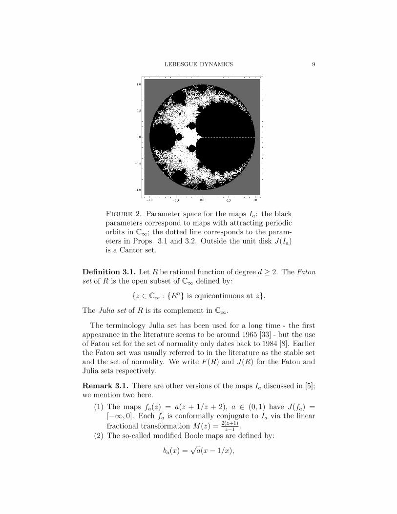
Figure 2. Parameter space for the maps Ia

: the blackparameters correspond to maps with attracting periodicorbits in C1; the dotted line corresponds to the param-eters in Props. 3.1 and 3.2. Outside the unit disk J(I

a

)is a Cantor set.

Definition 3.1. Let R be rational function of degree d � 2. The Fatouset of R is the open subset of C1 defined by:

{z 2 C1 : {Rn} is equicontinuous at z}.

The Julia set of R is its complement in C1.

The terminology Julia set has been used for a long time - the firstappearance in the literature seems to be around 1965 [33] - but the useof Fatou set for the set of normality only dates back to 1984 [8]. Earlierthe Fatou set was usually referred to in the literature as the stable setand the set of normality. We write F (R) and J(R) for the Fatou andJulia sets respectively.

Remark 3.1. There are other versions of the maps Ia

discussed in [5];we mention two here.

(1) The maps f

a

(z) = a(z + 1/z + 2), a 2 (0, 1) have J(fa

) =[�1, 0]. Each f

a

is conformally conjugate to I

a

via the linearfractional transformation M(z) = 2(z+1)

z�1 .(2) The so-called modified Boole maps are defined by:

b

a

(x) =pa(x� 1/x),

10 JANE HAWKINS

taking the positive square root of a 2 (0, 1). Each f

a

is a fac-tor of the modified Boole map b

a

, via the two-fold branchedcovering map �(x) = �x

2.

In Fig. 2 we see that the parameters a 2 (0, 1) form the axis ofa cardioid; this parameter space appeared in ([28], Fig. 11) and hasbeen studied by the author in [18]. In particular the black areas of theparameter space represent open sets of parameters where an attractingperiodic orbit exists. There are other areas of Fig. 2 that give mapsof great interest in the study of Lebesgue dynamics. For example, westudy a map corresponding to a non-real parameter, whose Julia set isthe entire sphere, in Section 4. We now turn to the parameter a = �1,which generalizes to another parametrized family of quadratic maps,one whose only intersection with the space shown in Fig. 2 is that onepoint.

Proposition 3.3. We define the map I(z) ⌘ I�1(z). We have I :R[{1} ! R\(�2, 65), and I has the following properties as a rationalmap on C1:

(1) I(z) = �(8+6z2)4�5z2 has fixed points at 2 and �2

5 ±45i.

(2) I 0(2) = �1 and the other two fixed points are repelling.(3) There are no period 2 cycles for I; i.e., the fixed points of I2

are 2, 2, 2,�25 +

45i and �2

5 �45i.

Proof. One can check the fixed points and their derivatives by usingProp 3.1. Solving for period 2 points of I is equivalent to finding theroots of the polynomial j(z) = 5z5�26z4+40z3�16z2+16z�32; usinglong division one can easily determine that j(z) = (z�2)3(5z2+4z+4),from which the result follows. ⇤

It is also stated in ([28], caption of Fig. 6) that a quadratic rationalmap has a fixed point with derivative �1 if and only if it has no periodtwo orbits. This is proved in [17] along with a complete classification ofwhich rational maps of degree d lack periodic orbits of period k; mostof these maps result in nonsmooth Julia sets. However the quadraticfamily contains some examples of interest. The study of rational mapsmissing periodic orbits of certain periods goes back to Baker [3] andexamples are given in [7]. Hagihara gave a complete list of such mapsin her Ph.D. thesis [17].

Corollary 3.2. [17] The map I is conformally conjugate to a map of

the form:

(5) S

↵

(z) =z

2 � z

1 + ↵z

,

LEBESGUE DYNAMICS 11

for some ↵ 2 C \ {1}.

Proof. It is proved in [17] that a quadratic map has no period 2 cyclesif and only if it is conformally conjugate to a map of the form (5). ⇤

While J(I) is fractal and does not have nice Lebesgue measurableproperties (meaning with respect to m2,m1 or `), the family of mapsS

↵

, which includes a conformally conjugate copy of I, leads us to ourdiscussion about infinite measure preserving maps.

3.1. A family of ergodic and exact rational maps with an in-finite �-finite invariant measure equivalent to `. In this sectionwe turn to infinite Lebesgue measure ` on R. We have so far looked atfamilies of finite measure preserving examples. There are maps withsmooth one-dimensional Julia sets with the property that they pre-serve an infinite ergodic and exact �-finite measure equivalent to m.Therefore they cannot preserve an equivalent ergodic finite measure soare fundamentally di↵erent from the family given in Eqn (4). We nowreturn to the family of maps from Eqn (5): S

↵

(z) = z

2�z

1+↵z

, and we areinterested only in ↵ < �1 for now.

The next modification we make is to conjugate S↵

by the involution�(z) = 1/z, which gives us a map of the form:

(6) U1+↵

(z) = �z � 1 + ↵

z � 1� (1 + ↵).

If ↵ < �1, then U1+↵

is called a negative R-function; it can alsobe thought of as the square root of an inner function in the followingsense. Recall that an inner function is a map f of the upper halfplane satisfying: lim

y!0 f(x + iy) = f(x), for ` a.e. x 2 R. Thedynamics of inner functions have been studied extensively by Aaronson[1], along with the criteria supplied by Letac [25] on when they (andrational negative R-functions) preserve the infinite measure ` on R. Itis also directly verifiable that U

↵

preserves Lebesgue measure on R.Rational maps that are negative R-functions flip the upper and lowerhalf plane, but every even iteration is an inner function, so U

21+↵

isan inner function. To simplify notation, we write b = 1 + ↵, and werestrict to ↵ 2 [�3,�1) (see [7, 17]); for any ↵ < �3 , S

↵

is conformallyconjugate to S 3�↵

1+↵; then b 2 [�2, 0). For the next two theorems we need

to recall the following concepts from infinite measure dynamics.

Remark 3.2. (1) Since U

b

preserves ` on R, (for b < 0), and ` isinfinite, for any fixed c > 0, U

b

also preserves the scaled measuregiven by (c `)(A) ⌘ c · `(A) for all measurable A. We say the

12 JANE HAWKINS

maps Ub1 and U

b2 are c-isomorphic if for some c > 0, there existsa measurable isomorphism � : R ! R with �⇤` ⌘ `���1 = (c `),and such that � � U

b1 = U

b2 � �, ` - a.e.(2) Assume A ⇢ R satisfies 0 < `(A) < 1 and `(R\[1

i=0U�i

b

(A)) =0. Then replacing U

b

by U for simplicity of notation, by U

A

we mean the map on A given by: U

A

(x) = U

p(x)(x) wherep(x) = min{i : U i(x) 2 A}.

(3) Since U preserves `, (2) defines a measure preserving endomor-phism U

A

: (A,B \ A, `|A

) ! (A,B \ A, `|A

) where `|A

denotesthe (non normalized) restriction of `. We call U

A

the induced

map on A.

We have the following results from the Ph. D. thesis of Bayless [6];(1) was shown in [17].

Theorem 3.3. [6] For b 2 [�2, 0), for the map U

b

(z) = �z � b+ b

1�z

,

the following hold with respect to `:

(1) J(Ub

) = R [ {1} ;

(2) U

b

is conservative, exact, and ergodic;

(3) For each U

b

, there exists a set A 2 B of finite measure such that

for `-a.e. x 2 R there exists a p(x) 2 N such that U

p(x)b

(x) 2 A,

and such that the first return time partition (to A) of R has

finite entropy (i.e., U

b

is said to be quasi-finite).

3.1.1. Entropy on infinite spaces. We assume the reader has familiar-ity with the notion of measure theoretic entropy on probability spaces,and if not, Walters’ book ([37], Chap 4) is a good source. When deal-ing with infinite invariant measures, there is an issue of scaling by aconstant, which can change the value of invariants; here we use ` on R,so `([0, 1]) = 1. The earliest definition of entropy of an infinite measurepreserving transformation is due to Krengel and is given as follows:

Definition 3.2. [22] If T : (X,B, µ) ! (X,B, µ) is a conservativemeasure-preserving system, then we define the Krengel entropy of Tby:

hkr(T ) = suph(TA

, µ

A

),

where the supremum is taken over all A 2 B satisfying 0 < µ(A) < 1.We denote the Krengel entropy of U

b

with respect to Lebesgue measure` on R, by hkr(Ub

).

From Theorem 3.3 the Krengel entropy of each U

b

is defined, andcan be calculated for the maps U

b

.

LEBESGUE DYNAMICS 13

Theorem 3.4. [6] For each b 2 [�2, 0),

hkr(Ub

) =

Z

Rlog |U 0

b

(t)|d`(t) = 2⇡p�b.

Moreover Bayless showed that every map of the form: f(z) = �z ��� p

t� z

, with �, t 2 R, and p > 0 (i.e., any quadratic rational negative

R-function), is c-isomorphic to exactly one map in the family U

b

, andU

b

and U

b

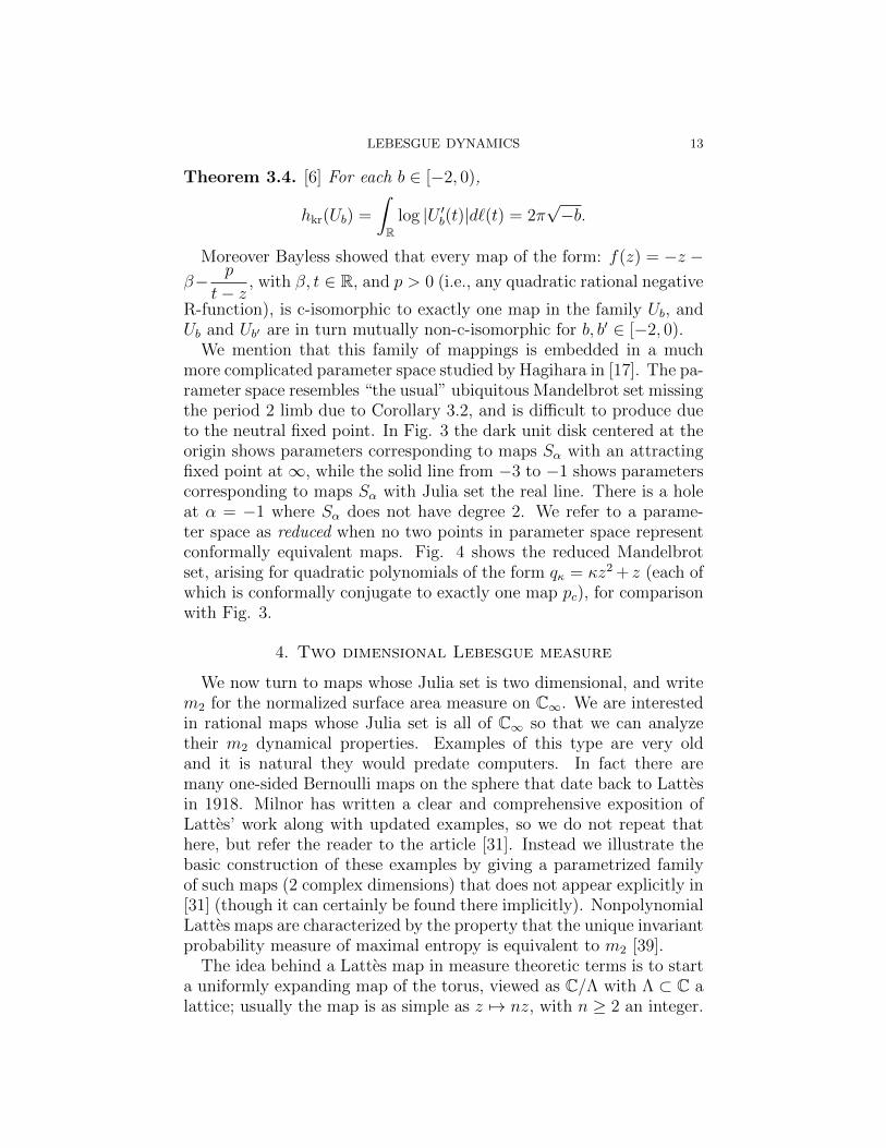
0 are in turn mutually non-c-isomorphic for b, b0 2 [�2, 0).We mention that this family of mappings is embedded in a much

more complicated parameter space studied by Hagihara in [17]. The pa-rameter space resembles “the usual” ubiquitous Mandelbrot set missingthe period 2 limb due to Corollary 3.2, and is di�cult to produce dueto the neutral fixed point. In Fig. 3 the dark unit disk centered at theorigin shows parameters corresponding to maps S

↵

with an attractingfixed point at 1, while the solid line from �3 to �1 shows parameterscorresponding to maps S

↵

with Julia set the real line. There is a holeat ↵ = �1 where S

↵

does not have degree 2. We refer to a parame-ter space as reduced when no two points in parameter space representconformally equivalent maps. Fig. 4 shows the reduced Mandelbrotset, arising for quadratic polynomials of the form q

= z

2+ z (each ofwhich is conformally conjugate to exactly one map p

c

), for comparisonwith Fig. 3.

4. Two dimensional Lebesgue measure

We now turn to maps whose Julia set is two dimensional, and writem2 for the normalized surface area measure on C1. We are interestedin rational maps whose Julia set is all of C1 so that we can analyzetheir m2 dynamical properties. Examples of this type are very oldand it is natural they would predate computers. In fact there aremany one-sided Bernoulli maps on the sphere that date back to Lattesin 1918. Milnor has written a clear and comprehensive exposition ofLattes’ work along with updated examples, so we do not repeat thathere, but refer the reader to the article [31]. Instead we illustrate thebasic construction of these examples by giving a parametrized familyof such maps (2 complex dimensions) that does not appear explicitly in[31] (though it can certainly be found there implicitly). NonpolynomialLattes maps are characterized by the property that the unique invariantprobability measure of maximal entropy is equivalent to m2 [39].

The idea behind a Lattes map in measure theoretic terms is to starta uniformly expanding map of the torus, viewed as C/⇤ with ⇤ ⇢ C alattice; usually the map is as simple as z 7! nz, with n � 2 an integer.

14 JANE HAWKINS

Figure 3. Parameter space for the maps S

↵

, equiva-lently U

b

, with `- preserving maps from Thm 3.3 markedby a solid (blue) line. The dashed (red) circle enclosesthe reduced parameter space.

Figure 4. Reduced parameter space for the mapsq

(z) = z+z

2, known as the Mandelbrot set. (Comparethis with Fig. 3).

LEBESGUE DYNAMICS 15

Such a map is easily seen to be ergodic, preserves `2, two dimensionalLebesgue measure on C/⇤, and the generating partition to make itone-sided Bernoulli (i.e., isomorphic to the one-sided { 1

n

2 ,1n

2 , . . . ,1n

2}shift) is obvious. We then find a suitable factor map from the torusto the sphere, and look at the map generated on C1. If the factormap is finite-to-one, the pullback measure will inherit the Bernoullimeasurable properties.

We also discuss postcritically finite maps that are not Lattes maps,and give the idea behind the result that such maps admit an ergodicfinite invariant measure equivalent to m2. There are many open ques-tions about their measure theoretic entropy as well as the Hausdor↵dimension of the maximal entropy measure whose support is necessarilythe entire sphere.

4.1. A family of Lattes examples of degree 4. We begin with acomplex torus: Let �1,�2 2 C\{0} with �2/�1 /2 R. A lattice is definedby ⇤ = [�1,�2] : = {m�1 + n�2 : m,n 2 Z}; ⇤ is a discrete additivesubgroup of C of rank 2, so C/⇤ is a torus. Di↵erent sets of vectorscan generate the same lattice ⇤, but if ⇤ = [�1,�2], and

⇤ = [�3,�4], the generators are related by✓�3

�4

◆=

✓a b

c d

◆✓�1

�2

◆

with a, b, c, d 2 Z and ad � bc = ±1. Therefore given any lattice⇤ = [�1,�2], we interchange the order if needed, so that

⌧ = �2/�1 2 H = {z : z = x+ iy, y > 0}.

It is useful to define an equally proportioned lattice ⌦ = [1, ⌧ ], and set

(7) ⇤ = k⌦ = k[1, ⌧ ], ⌧ 2 H, k 6= 0.

A simple map such as L(z) = ↵z, with the property that ↵⇤ ⇢ ⇤and |↵| > 1 defines a uniformly expanding map on C/⇤ which gives risevia a meromorphic factor map to a rational map of C1 of degree ↵2.We use n = 2 in the family of examples in Theorem 4.1, and integersn � 2 are the easiest to work with; however there are infinitely manynoninteger examples, and in Fig. 2, at the parameter a = �1

4 we have

a Lattes example obtained by using ⇤ = [1, i] and ↵ =p2.

The factor map we use for these examples is an elliptic functionwhich, by definition, is a meromorphic function in C periodic withrespect to a lattice ⇤. In our examples we use the Weierstrass elliptic

16 JANE HAWKINS

} function, defined by

}⇤(z) =1

z

2+

X

w2⇤\{0}

✓1

(z � w)2� 1

w

2

◆, z 2 C.

Replacing every z by �z in the definition we see that }⇤ is an evenfunction, }⇤ is meromorphic, periodic with respect to ⇤, and eachpole, occurring exactly at lattice points, has order 2. The function }exhibits some characteristics of trigonometric functions; it is periodic(with respect to a rank 2 subgroup of C rather than rank 1), it isrelated to its own derivative via a simple di↵erential equation (see Eqn(8) below), and we have an “angle doubling” formula (see Eqn (12)below).

4.1.1. ODEs for }⇤ and its derivatives: We have

(8) }

0⇤(z)

2 = 4}⇤(z)3 � g2}⇤(z)� g3,

where

(9) g2(⇤) = 60X

w2⇤\{0}

1

w

4and g3(⇤) = 140

X

w2⇤\{0}

1

w

6.

Remark 4.1. We call (g2, g3) invariants of ⇤ ([13], Chap 2.22). Inparticular g2(⇤) and g3(⇤) are complete invariants of the lattice ⇤ sincefor any g2 and g3 such that g32 � 27g23 6= 0 there exists a unique latticehaving g2 and g3 as its sums in Eqn(9), ([13], Chap 2.11, and [21],Cor. 6.5.8), or equivalently, the pair (g2, g3) determines completely thevalue of }⇤(z) for all z 2 C. Moreover the invariants g2, g3 dependanalytically on ⇤ in the sense that they vary analytically in ⌧ 2 Hwhen represented as in Eqn (7) (see [21], Thm 6.4.1), and from Eqn(9) it follows that

(10) g2(k⌦) = k

�4g2(⌦), and g3(k⌦) = k

�6g3(⌦).

Analogous to sine and cosine functions, we also have a second orderODE connecting the second derivative to the original function:

(11) }

00⇤(z) = 6}2

⇤(z)�g2

2.

4.1.2. Angle Doubling Formula for }⇤:

(12) }⇤(2z) =}

00⇤(z)

2

4}0⇤(z)

2� 2}⇤(z).

These classical identities and many others are worked out in detailin [13] or [21]. Putting together Eqns. (8) - (12), via the commuting

LEBESGUE DYNAMICS 17

diagram below, we obtain a rational map of the sphere of the form:

(13) R(z) =z

4 + (g2/2)z2 + 2g3z + g

22/16

4z3 � g2z � g3,

depending on ⇤(g2, g3).

(C/⇤,B, `2) 2z�! (C/⇤,B, `2)# }⇤ # }⇤

C1R�! C1

Since }⇤ is meromorphic, the pullback measure on C1, (}⇤)⇤`2, isequivalent to m2. We are now ready to state our theorem, and give abrief proof.

Theorem 4.1. Given any 3 distinct complex numbers, a, b, c such that

a+ b+ c = 0, there exists a rational map of degree 4 of the form:

(14) R(z) =z

4 + (↵/2)z2 + 2�z + ↵

2/16

4z3 � ↵z � �

with ↵, � 6= 0, such that:

(1) J(R) = C1(2) The critical values of R are exactly a, b, and c, each of multi-

plicity 2.(3) The critical values get mapped to a fixed point at 1, which is

repelling.

(4) There are 6 distinct critical points for R, and they sum to 0.(5) There exists a lattice ⇤ such that }⇤ induces the map R from a

toral endomorphism on C/⇤;(6) The map R is isomorphic to the one-sided {1

4 ,14 ,

14 ,

14} Bernoulli

shift with respect to the invariant probability measure µ = (}⇤)⇤`2 ⇠m2.

Proof. Given a, b, c we reorder them if necessary so that a 6= 0, b 6= 0;recall that at most one can be 0, so we assign that value to c if it occurs.We next set p(z) = (z � a)(z � b)(z � c) and write it as:

p(z) = (z� a)(z� b)(z� (�a� b)) = z

3 � (a2 + ab+ b

2)z+(a2b+ ab

2).

Using the angle doubling identities we get: ↵ = 4(a2+ab+b

2), � =�4(a2b+ ab

2) to obtain

R(z) =z

4 + (↵/2)z2 + 2�z + ↵

2/16

4z3 � ↵z � �

18 JANE HAWKINS

While the statements about the critical values follow from some iden-tities, in this case they can also be verified by hand. In particular,the 6 critical points for the map R are: a ±

p2a2 � ab� b

2, b ±p�a

2 � ab+ 2b2, and c ±p2a2 + 5ab+ 2b2, which sum to 0. The

discriminant given for each critical point does not vanish because a, b,and c are distinct. Using g2 = ↵ and g3 = �, we find a unique lattice⇤(g2, g3) which we use for the covering torus. ⇤

It is not hard to vary the theorem a little in order to specify thatc1, c2 = ±q 2 C be (distinct) critical points, instead of specifying thecritical values. Choosing g2 = 4( q

1+p2)2 and g3 = 0 in (13) will work.

4.2. An example illustrating Theorem 4.1. In Theorem 4.1, wechoose any nonzero a 2 C, b = �a, and c = 0. Following the proof, wesee that ↵ = 4(a2+ab+b

2) = 4a2 (which is g2), and � = �4(a2b+ab

2) =0 (which is g3), yielding the rational map:

(15) F (z) =z

4 + 2a2z2 + a

4

4z(z2 � a

2).

It is a calculation to show that the 6 critical points for F are: ±ai, a(1±p2), a(�1±

p2). The critical values are as follows: F (ai) = F (�ai) =

0. One can substitute the other critical points and see that

F (a+a

p2) = F (a�a

p2) = a and F (�a+a

p2) = F (�a�a

p2) = �a;

so we recover the three distinct critical values. It is then easy to seethat each of the critical values has multiplicity 2 and is a pole, so ismapped under f to 1 2 C1.

The four fixed points for F that are in C, are:

±ai

s

�1 +2p3, ±a

s

1 +2p3,

and F

0(x) = �2 for each of the fixed points. We note that 1 is also afixed point, and we calculate its multiplier, the analog of a derivativeat 1 when C1 is viewed as a compact surface. This is the derivativeof: z 7! 1/f(1

z

) at the origin, which can be shown to be 4.Moreover every periodic point of period k, has derivative ±2m for

some positive integer m, and in this example m = k or m = 2k foreach k. This is a characteristic of Lattes examples, that their periodicpoints have derivatives of a particular form, but not verifiable unlessyou know how you arrived at the example (in our case, by multiplicationby 2 on the torus, and then used } as the factor map). This is discussedin ([31], Cor. 3.9).

LEBESGUE DYNAMICS 19

Using Eqn.(10) we see that when b = �a, the underlying lattice ⇤coming from Theorem 4.1 is of the form ⇤ = [�,�i], � 6= 0 satisfying

� =1pa

· �,

where � > 0 is the lemniscate constant which arises as the lattice sidelength for invariants g2 = 4, g3 = 0. Many details behind the constant� and the invariants g2, g3 are discussed in [19].

4.3. Postcritically finite rational maps. The Lattes examples arespecial cases of postcritically finite rational maps. By definition, arational map is postcritically finite if every critical point is preperiodicbut not periodic. This excludes maps like X

d

(z) = z

d, where 0 and 1are both fixed critical points on C1, but includes maps like the one inExample 4.2 and more general maps. We define the postcritical set ofR by:

(16) P (R) =[

c2C(R), n2N

R

n(c),

where C(R) is the set of critical points of R; by definition P (R) isclosed and may or may not contain points from C(R).

The reason a postcritically finite map R is of interest in Lebesgueergodic theory is that J(R) = C1; a proof of this can be found in manyplaces (see [7], Thm 9.4.4), but the basic idea is that any time thereis a Fatou component, it maps eventually to a periodic componentwhich must have a critical point associated to it (either in the Fatouset or with an infinite forward orbit, or both). This means that itis worth considering the measure theoretic structure of a postcriticallyfinite map R with respect to the 2-dimensional probability measurem2,as each such map is always topologically transitive (see e.g. [7], Thm4.2.5). The measurable dynamics of postcritically finite maps have beenextensively written about (e.g., [4, 14, 18, 27, 34]) and generalized toother settings (meromorphic postcritically finite, entire postcriticallyfinite, and rational maps not postcritically finite but “close” to one).Here we review only a few of the basic measure theoretic results.

Remark 4.2. (1) Assume that P (R) = {a1, a2, . . . , ak} with eacha

j

/2 C(R); it follows that |P (R)| � 3 ([27], Thm 3.6). To eacha

j

we assign the positive integer ⌫j

which is the least commonmultiple of the local degrees deg(Rk

, y), for all k > 0 and y suchthat y 2 R

�k(x). We then have a set of ramification indices:N = {⌫1, ⌫2, . . . , ⌫k} with each ⌫

k

� 2. This leads to a metricwhich has a finite set of singularities for an otherwise smooth

20 JANE HAWKINS

Riemannian metric ⇢ = �(z)|dz| on C1, and the singularities

are of the type ⇢ =|dz|

|z|1�1/⌫jin local coordinates near each a

j

.

(2) The pair (C1 \ P (R),N ), with a complex atlas structure onC1 \ P (R), is called the orbifold of R and the metric ⇢ is itsassociated orbifold metric.

An application of the Schwarz lemma to the covering space of theorbifold C1 \P (R), which is the disk with the hyperbolic metric since|P (R)| � 3, gives the following result. Details can be found in any oneof these sources ([14, 27, 30])

Theorem 4.2. [14] A postcritically finite map R is expanding with

respect to its orbifold metric and kR0(z)k > � > 1 for all z 2 C1\P (R).

The next result is a compendium and a simplification of results bymany authors. We cite a few places where the statements can be found,more or less as stated here; most of these results were shown by Rees[34].

Theorem 4.3. If R is a postcritically finite rational map then the

following hold.

(1) R is ergodic, exact, and conservative with respect to m2 [4, 27,34];

(2) R admits an invariant probability measure ⌫ ⇠ m2 [34].(3) Let M be a connected 1 complex dimensional manifold, and

suppose {Ra

, a 2 M} is a parametrized family of rational map-

pings that vary holomorphically in a; assume there exists some

a0 2 M such that R

a0 is postcritically finite. If R

a

satisfies

a nondegeneracy condition (given in Remark 4.3 below), then

there exists a set of parameters of positive measure in M such

that (1) and (2) hold [34].

Remark 4.3. (1) Polynomials never satisfy the hypotheses of The-orem 4.3 since the point at 1 is a fixed critical point for everypolynomial. The examples and results from Sec. 3.1, S

↵

andU

b

, can never be post critically finite either since a parabolicfixed point forces a map to have an infinite forward orbit (see[7], Thm 9.3.2).

(2) The nondegeneracy condition in Theorem 4.3 is described as fol-lows. Fix the postcritically finite parameter a0. By consideringa higher iterate of R

a

if necessary, assume each critical orbit ter-minates in a (necessarily repelling) fixed point. Assume the mapR

a0 has critical points c1(a0), . . . , cm(a0), m 2d�2. Write the

LEBESGUE DYNAMICS 21

fixed point at the end of the orbit of ci

(a0) as: R

si(ci

(a0)) =y

i

(a0) = R

a0(yi(a0)) = z

i

(a0) for each i = 1, . . . ,m, wheres

i

= min{k : Rk(ci

(a0)) is fixed}.Each of these points moves holomorphically in a 2 M. The

nondegeneracy condition is that the function:

F

i

(a) = R

si+1(ci

(a))�R

si(ci

(a))

should satisfy:

(17)DF

i

Da

(a0) 6= 0,

or equivalently,

Dz

i

Da

(a0)�Dy

i

Da

(a0) 6= 0.

(3) We give an example of a family of maps satisfying the non-

degeneracy condition, from [34]. If Ra

(z) = a

(z � 2)2

z

2, with

a 2 C \ {0} then the critical points are c1 = 0 and c2 = 2, andthe critical orbits look like:

2 7! 0 7! 1 7! a 7! (a� 2)2

a

· · ·

We set R

a

(a) = a, and note that R

0a

(a) = 4(a�2)a

2 . Thereforechoosing a0 = 1, yields both critical orbits terminating at arepelling fixed point at 1. We can check the condition in Eqn(17) by brute force to see that both resulting derivatives yield�4 6= 0.

(4) The family of maps shown in Fig. 2, which we write as: fa

(z) =a(z + 1/z + 2), has a fixed critical orbit at c1 = �1. Namely�1 7! 0 7! 1 for all nonzero a. The multiplier of the fixedpoint at 1 is 1/a, so as long as a stays in the open unit diskD of parameters, this is a repelling fixed point. Therefore weonly look at the second critical point, c2 = 1 to check the non-degeneracy condition given by (17); the purpose of Condn (17)in [34] is to estimate the measure of the set of parameters onwhich both critical orbits “stay far enough away from” criticalpoints, which is una↵ected by only checking for c2. If we seta0 =

�3�p7i

8 , we see that under fa0 ,

1 7! �3�p7i

27! �3 +

p7i

8,

and z0 =�3+

p7i

8 is fixed. Moreover |f 0a0(z0)| = |1/a0| = 2.

22 JANE HAWKINS

Using the notation in (1),

F2(a) = f

2a

(1)� f

a

(1) =(1 + 4a)2

4� 4a =

(1� 4a)2

4,

and DF2Da

(a0) = �5 �p7i 6= 0 when a0 = �3�

p7i

8 . This im-plies that the family of map I

a

, defined by Eqn (4), whenparametrized over a 2 C contains a set of parameters of positiveLebesgue measure for which J(I

a

) = C1 and for which Thm4.3 holds. This is mentioned in [18].

(5) Apart from the Lattes examples we do not look for parametrizedfamilies of rational maps whose Julia set is the whole sphere;they are very unstable mappings, and in a neighborhood of aparameter of a postcritically finite map one usually sees othersimilar maps as well as tiny Mandelbrot sets signaling the pres-ence of maps with attracting orbits (see [18, 27] for example).

4.4. Recent results: fractal Julia sets of positive m2 measure.In this section we review some recent results about the existence ofquadratic polynomials whose Julia sets have positive m2 measure [12].We have a limited goal here of giving the reader an idea of how apositive Lebesgue measure Julia set could possibly arise. This result,Theorem 4.4 below, is quite remarkable and represents a creative andtechnical leap forward in the field. Like many good ideas, the basicconstruction can be explained in simple terms. And also like manysignificant breakthroughs the process of arriving at the constructioninvolved many people, di�cult technical tools (e.g., [20]), and a lot ofgroundwork before the key idea fell into place. The result appears in apaper by Bu↵ and Cheritat [12] but their introduction mentions manycontributions by others. Background material for this section can befound in [29].

We start by recalling the familiar definition of a filled Julia set of apolynomial map p(z): namely,

(18) K(p) = {z 2 C : {pn(z)}n2N is bounded}.

We consider the family of quadratic polynomials parametrized as:

(19) q

(z) = z + z

2, 2 C.

In this form we see immediately that 0 is a fixed point with multiplier. For the construction we are only interested in || = 1, and moreprecisely in = e

2⇡i⇠ with ⇠ an irrational number, so we replace thenotation q

e

2⇡i⇠ with q

⇠

. We refer to 0 as an irrationally indi↵erent fixedpoint, and these points are of two types: either 0 is a Siegel point if

LEBESGUE DYNAMICS 23

there exists a local holomorphic change of coordinate z = �(w) suchthat:

q

⇠

� �(w) = � � e2⇡i⇠wfor all w near the origin, or it is a Cremer point if no such local mapexists. While irrational numbers giving Siegel points for q

⇠

have fullLebesgue measure in [0, 1], Cremer point values of ⇠ form a dense G

�

set. The rotation numbers that occur for Siegel disks are relativelypoorly approximable by rational numbers while the Cremer numbersare well approximable. Siegel points give rise to maps that have a Fatoucomponent containing 0, so that q

⇠

is locally conjugate to rotationthrough 2⇡⇠ on a disk. In Fig. 5 we show a Siegel disk. By contrast,Cremer points are always in the Julia set of q

⇠

.In general, if J(p) is connected, @K(p) = J(p) ( K(p), but it can

happen, as is shown in Fig. 6 that K(p) has empty interior and isJ(p). If one starts with irrational numbers that have Siegel disks, andthen takes a sequence ⇠

n

that has been carefully chosen so that theLebesgue measure of K(q

⇠n+1) stays close to the measure of K(q⇠n),

then a limiting value ⇣ might appear which is not a Siegel number,but m2(K(q

⇣

)) > 0 and K(q⇣

) = J(q⇣

). This is roughly how theconstruction goes, after showing that the map ⇠ 7! m2(K(q

⇠

)) is uppersemicontinuous. In other words, the authors are able to construct ⇠

n

!⇣ with these (and more) properties.

Theorem 4.4. [12]

• There exist quadratic polynomials that have a Cremer fixed point

and a Julia set of positive m2 measure.

• There exist quadratic polynomials which have a Siegel disk and

a Julia set of positive m2 measure.

Some topological properties of the Julia sets resulting from this workhave been published (see [9] for example.) Since there exists a uniqueinvariant probability measure µ supported on the Julia set such thath

µ

(p) = log 2, and it must be singular with respect to m2 [39], theLebesgue measure properties of these maps are still largely unknown.

References

[1] Aaronson, J (1978) Ergodic theory for inner functions of the upper half plane.Ann. Inst. H. Poincar Sect. B (N.S.) 14, no. 3, 233 –253.

[2] Avila A, Bu↵ X, Cheritat A (2004) Siegel disks with smooth boundaries. ActaMath. 193, no. 1, 1–30.

[3] Baker I N, (1964) Fixpoints of polynomials and rational functions. J. LondonMath. Soc. 39, 615–622.

24 JANE HAWKINS

Figure 5. The map q

p7(z) = e

�2⇡ip7z + z

2 has a filledJulia set that is a Siegel disk centered at the fixed pointat z = 0.

-2 -1 1 2

-2

-1

1

2

Figure 6. For the map p�1(z) = z

2 + i, K(pi

) = J(pi

)

Figure 7. For the filled Julia set of the map q

⇠

(z) =e

2⇡i⇠z+z

2, a small perturbation in ⇠ can cut deeper fjordsin K(q); on the left ⇠1 = .131578 . . . and on the right,⇠2 = ⇠1 + " with " < .00125

LEBESGUE DYNAMICS 25

[4] Barnes, J (1999) Conservative exact rational maps of the sphere. J. Math.Anal. Appl. 230, no. 2, 350–374.

[5] Barnes J, Hawkins J (2007) Families of ergodic and exact one-dimensionalmaps, Dynamical Systems: An Intl. Jour., Vol. 22, no. 2, 203–217.

[6] Bayless R (2013) Entropy of Infinite Measure-Preserving Transformations,PhD thesis, University of North Carolina at Chapel Hill.

[7] Beardon A (1991) Iterations of Rational Functions, Springer-Verlag GTM 132.[8] Blanchard, P (1984) Complex analytic dynamics on the Riemann sphere. Bull.

Amer. Math. Soc. (N.S.) 11, no. 1, 85 –141.[9] Blokh A, Oversteegen, L (2006) The Julia sets of quadratic Cremer polynomi-

als. Topology Appl. 153, no. 15, 3038–3050.[10] Bruin H, Hawkins J (2001) Exactness and maximal automorphic factors of

unimodal interval maps, Erg. Th. and Dyn. Sys. 21,4, 1009 –1034.[11] Bruin H, Hawkins J (2009) Rigidity of Smooth One-Sided Bernoulli Endomor-

phisms, N.Y. Journal of Math, 15, 451-483.[12] Bu↵ X, Cheritat A (2012) Quadratic Julia sets with positive area. Ann. of

Math. (2) 176 (2012), no. 2, 673–746.[13] DuVal, P (1973) Elliptic Functions and Elliptic Curves, Cambrige Univ. press.[14] Ermenko A, Lyubich M (1990) The dynamics of analytic transformations.

(Russian) Algebra i Analiz 1 (1989), no. 3, 1–70; translation in LeningradMath. J. 1, no. 3, 563–634.

[15] Friedman N and Ornstein D (1970) On isomorphism of weak Bernoulli trans-formations, Adv. in Math 5, 365–394.

[16] Furstenberg H (1967) Disjointness in ergodic theory, Math. Sys. Theory 1,1–50.

[17] Hagihara R (2007) Rational Maps Lacking Certain Periodic Orbits. PhD thesis,University of North Carolina at Chapel Hill.

[18] Hawkins J (2003) Lebesgue Ergodic Rational Maps in parameter space, IntlJour of Bif. and Chaos, Vol. 13, No. 6, 1423–1447.

[19] Hawkins J, Koss L (2002) Ergodic properties and Julia sets of Weierstrasselliptic functions. Monatsh. Math., 137 no. 4: 273 – 300.

[20] Inou H, Shishikura M (2006) The renormalization for parabolic fixed pointsand their perturbation, preprint.

[21] Jones G, Singerman D (1997) Complex Functions: An algebraic and geometricviewpoint, Cambridge Univ. Press

[22] Krengel U (1967) Entropy of conservative transformations, Z. Wahrschein-lichkeitstheorie und Verw. Gebiete, 7:161–181.

[23] Ledrappier F (1981) Some properties of absolutely continuous invariant mea-sures on an interval, Erg. Th. and Dynam. Sys. 1 77–93.

[24] Ledrappier, F (1984) Quelques proprietes ergodiques des applications ra-tionnelles, C.R. Acad. Sci. Ser. I math 299 37–40.

[25] Letac G (1977) Which functions preserve Cauchy laws? Proc. Amer. Math.Soc., 67(2):277–286.

[26] Lyubich, M (1983) Entropy properties of rational endomorphisms of the Rie-mann sphere. Ergodic Theory Dynam. Systems 3, no. 3, 351–385.

[27] McMullen, C (1994) Complex dynamics and renormalization, Annals of Math-ematics Studies, 135. Princeton University Press, Princeton, NJ.

26 JANE HAWKINS

[28] Milnor J (1993) Geometry and dynamical of quadratic rational maps, Experi-mental Math 2, 37–83.

[29] Milnor, J (2000) On Rational Maps with Two Critical Points. ExperimentalMath. 9 480–522.

[30] Milnor J (2000) Dynamics in One Complex Variable, Friedr. Vieweg & Sohn,Verlagsgesellschaft mbH.

[31] Milnor J (2006) On Lattes maps, Dynamics on the Riemann sphere, 9–43, Eur.Math. Soc., Zurich.

[32] Misiurewicz M (1981) Absolutely continuous measures for certain maps of aninterval, Publ. I.H.E.S.,53, 17–51.

[33] Nishino T, Yoshioka T, (1965) Sur l’iteration des transformations rationnellesentires de l’espace de deux variables complexes. (French) C. R. Acad. Sci. Paris260, 3835–3837.

[34] Rees, M (1986) Positive measure sets of ergodic rational maps. Ann. Sci. coleNorm. Sup. (4) 19, no. 3, 383–407.

[35] van Strien, S (1990) Hyperbolicity and invariant measures for general C2 in-terval maps satisfying the Misiurewicz condition, Commun. Math. Phys. 128,437–496.

[36] Rohlin V (1963) Exact endomorphisms of a Lebesgue space, AMS Transl. Ser.2 39, 1–36.

[37] Walters P (1975) An Introduction to Ergodic Theory, Springer Grad Text inMath 79. Springer: NY.

[38] Yongcheng Y (1992) On the Julia sets of quadratic rational maps, Comp. Var.18, 141–147.

[39] Zdunik A (1990) Parabolic orbifolds and the dimension of the maximal measurefor rational maps, Invent. Math. 99, 627–649.

Department of Mathematics, University of North Carolina at ChapelHill, CB #3250, Chapel Hill, North Carolina 27599-3250

E-mail address: jmh@math.unc.edu