Least Square ++ Camera 3D Registration 3D triangulation...

Camera 3D Registration Perspective-n-Point Algorithm

LeastSquare++3Dtriangulation+cameraregistration

SlidesbyHyunSoo Park

1809,CarlFriedrichGauss

Singular Value Decomposition

A U= D VT

m x n m x n n x n n x n

U

Column orthogonal matrix

UTu= Im m VVT

u= In n

spans column space of A spans row space of A

Singular Value Decomposition

A U= D VT


U

Column orthogonal matrix

UTu= Im m VVT

u= In n

Singular value matrix

D , , ,= n"ı ı ı1 2diag{ } t t t tn"ı ı ı1 2 0where

Example I A = 0.9501 0.8913 0.8214 0.9218 0.2311 0.7621 0.4447 0.7382 0.6068 0.4565 0.6154 0.1763 0.4840 0.0185 0.7919 0.4057

[u,d,v] = svd(A) u = -0.7302 -0.1240 -0.1909 -0.6442 -0.4415 -0.6333 0.3797 0.5098 -0.3809 0.3258 -0.6565 0.5637 -0.3560 0.6910 0.6232 0.0859 d = 2.4475 0 0 0 0 0.6710 0 0 0 0 0.3652 0 0 0 0 0.1928 v = -0.4900 0.3993 -0.5212 -0.5734 -0.4771 -0.6432 -0.4626 0.3803 -0.5363 0.5428 0.2781 0.5835 -0.4946 -0.3636 0.6611 -0.4314

Example I A = 0.9501 0.8913 0.8214 0.9218 0.2311 0.7621 0.4447 0.7382 0.6068 0.4565 0.6154 0.1763 0.4840 0.0185 0.7919 0.4057

u*d*v' ans = 0.9501 0.8913 0.8214 0.9218 0.2311 0.7621 0.4447 0.7382 0.6068 0.4565 0.6154 0.1763 0.4840 0.0185 0.7919 0.4057

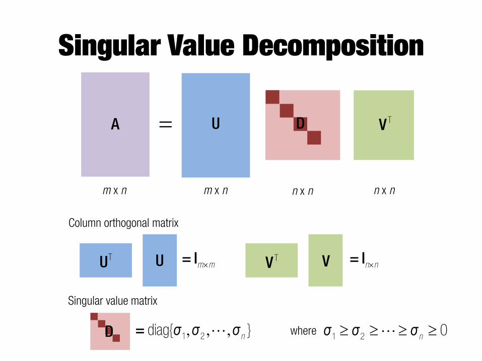
Reconstruction

SVDofthis?

U(:,1:4) D(1:4,1:4) V(:,1:4)’

[u,d,v]=svd(I); semilogy(diag(d(1:20,1:20)),'x-')

Im2=u(:,1:20)*d(1:20,1:20)*v(:,1:20)';

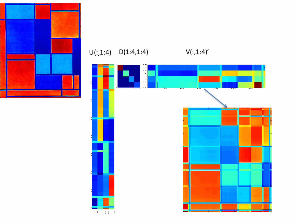
Images as Vectors

=

m

n

n*m

Vector Mean

=

m

n

n*m

=

n*m

I1 + I2 = mean image

Average face…

Eigenfaces

Eigenfaces look somewhat like generic faces.

Eigen-imagesofBerlin

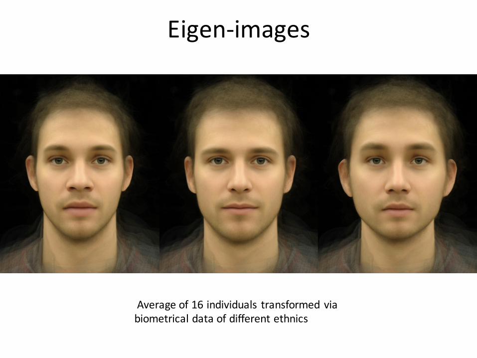
Eigen-images

Averageof16individuals transformedviabiometricaldataofdifferentethnics

Averageof16individuals transformedviabiometricaldataofdifferentages

Example II (Rotation)

XZ

23ʌș

� �e = + +1

3i j k ª º

« »« »« »¬ ¼

R =0 0 1

1 0 0

0 1 0

>> [u,d,v] = svd(R) u = 0 0 1 -1 0 0 0 -1 0 d = 1 0 0 0 1 0 0 0 1

v = -1 0 0 0 -1 0 0 0 1

Note that singular values are always one for a rotation matrix

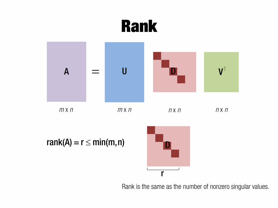
Rank

A U= D VT


drank(A) = r min(m,n) D

Rank is the same as the number of nonzero singular values.

r

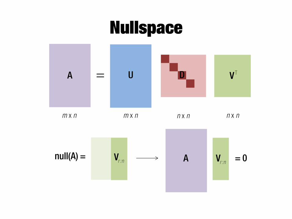
Nullspace

A U= D VT


null(A) = Vr :n Vr :nA = 0

Example III (Fundamental Matrix)

F = 1.0e+003 * -0.0000 0.0000 0.0030 -0.0001 0.0002 0.0564 0.0132 -0.0292 -9.9998

[u,d,v] = svd(F) u = -0.0003 0.9981 0.0618 -0.0056 -0.0618 0.9981 1.0000 -0.0001 0.0056 d = 1.0e+004 * 1.0000 0 0 0 0.0000 0 0 0 0.0000

v = 0.0013 -0.9660 0.2586 -0.0029 -0.2586 -0.9660 -1.0000 -0.0005 0.0032

d(1,1) ans = 1.0000e+004 d(2,2) ans = 0.0021 d(3,3) ans = 2.7838e-016

Rank(F) = 2

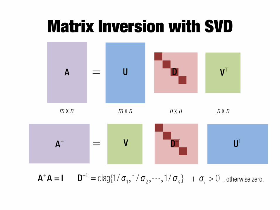
Matrix Inversion with SVD

A U= D VT


�A UT= �D 1V

1 , , ,�D = n"ı ı ı1 2diag{1/ 1/ 1/ } if , otherwise zero. !iı 0�A A = I

2

7

The SVD and Spectral Decomposition

Let A = UVT be an SVD

with = diag(�1, . . . , �c) and V = (v1 · · · vc)

We have that

the �i are the square root of the eigenvalues of ATA

the vi are the eigenvectors of ATA

Proof

ATA = VTUTUVT = V2VT 8

Kernel, Rank and the SVD

SVD0

A VU

T

The rank is 2

The left kernel has dimension 5� 2 = 3

The right kernel has dimension 3� 2 = 1

Basis for the right kernel

Partial basis for the left kernel

F Vector x is in the right kernel of A i& Ax = 0

F Vector y is in the left kernel of A i& yTA = 0T

F The rank k of matrix A is the number of nonzero singular values(0 � k � min(r, c))

F The right kernel has dimension c� k

F The left kernel has dimension r � k

9

Linear Least Squares (LLS) Optimization: Problem Statement

minx;Rn

kAx� bk2 s.t. C(x) = 0

minx;Rn

mX

j=1

¡aTj x� bj

¢2s.t. C(x) = 0

A(m×n) =

C

hhH

.

.

.

aTj...

I

nnO and b(m×1) =

C

hhH

.

.

.

bj...

I

nnO

m ‘equations’ and n ‘unknowns’

‘constraints’ means both ‘equations’ and ‘unknowns’ and is thus ambiguous

10

A Bit of History…

� 1795 – discovery of Least Squares by Gauss� 1801 – used by Gauss in astronomical calculations

(prediction of the orbit of the asteroid Ceres)� 1805 – publication of an algebraic procedure by

Legendre (dispute with Gauss)� The method quickly became the standard procedure

(for analysis of astronomical and geodetic data)� 1809, 1821, 1823 – statistical justification by Gauss� 1912 – rediscovery by Markov

11

Why Least Squares?

� Assume the noise on b is Independently and Identically Distributed (i.i.d.)

� Least Squares gives the Best Linear Unbiased Estimator (BLUE) – best = minimum variance

� Assume further that the noise on the data follows a gaussian distribution

� The Maximum Likelihood Estimator (MLE) is obtained by Least Squares

12

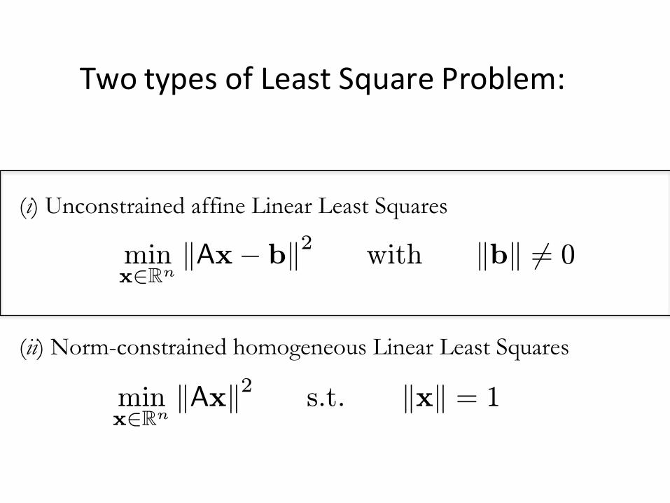
Two Cases of Interest

� (i) Unconstrained affine Linear Least Squares

� (ii) Norm-constrained homogeneous Linear Least Squares

� Notes� Both problems frequently appear in Computer Vision

(and in scientific computing in general)� (ii) handles (i) while (i) does not always handle (ii)

minx;Rn

kAx� bk2 with kbk 6= 0

minx;Rn

kAxk2 s.t. kxk = 1

TwotypesofLeastSquareProblem:

Least squares methods- fitting a line -

• Data: (x1, y1), …, (xn, yn)

• Line equation: yi = m xi + b

• Find (m, b) to minimize

¦ ��

n

i ii bxmyE1

2)(

(xi, yi)

y=mx+b

SilvioSavarese

022 � YXXBXdBdE TT

> @ 2

2

n

1

n

1n

1i

2

ii XBYbm

1x

1x

y

y

bm

1xyE � »¼

º«¬

ª

»»»

¼

º

«««

¬

ª�

»»»

¼

º

«««

¬

ª ¸̧

¹

·¨̈©

§»¼

º«¬

ª� ¦

��

Normal equation

¦ ��

n

i ii bxmyE1

2)(

YXXBX TT


� � YXXXB T1T �

)XB()XB(Y)XB(2YY)XBY()XBY( TTTT ��

SilvioSavarese

=

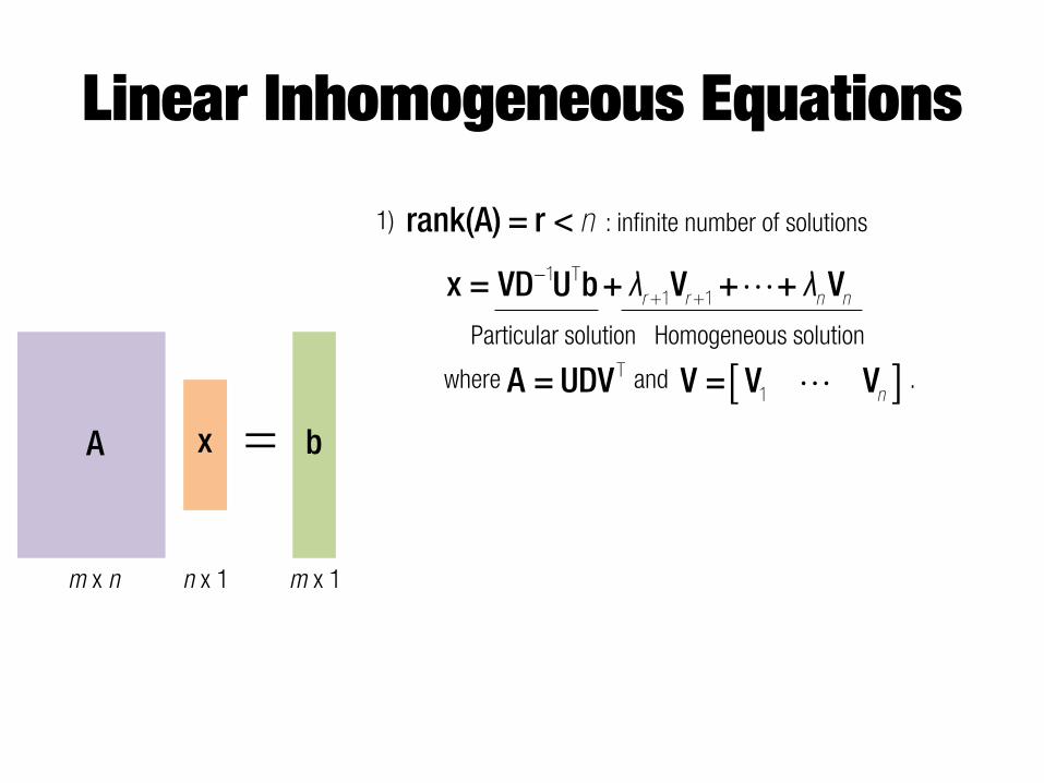
Linear Inhomogeneous Equations

A x b

m x n n x 1 m x 1

rank(A) = r < n : infinite number of solutions

�x = VD U b+ V + + Vr r n n"Ȝ Ȝ1 T+1 +1

Particular solution Homogeneous solution

where and . A = UDV T > @V = V Vn"1

1)

=


A x b

m x n n x 1 m x 1


rank(A) = n : exact solution

�x = VD U b+ V + + Vr r n n"Ȝ Ȝ1 T+1 +1



�x = A b1

1)

2)

=


A x b

m x n n x 1 m x 1


rank(A) = n : exact solution

�n m : no exact solution in general (needs least squares)

�x = VD U b+ V + + Vr r n n"Ȝ Ȝ1 T+1 +1



�x = A b1

� �x = A A A b-1T T

xmin Ax -b 2

Î

or in MATLAB. x = A \ b

1)

2)

3)


• Data: (x1, y1), …, (xn, yn)

• Line equation: yi = m xi + b

• Find (m, b) to minimize

¦ ��

n

i ii bxmyE1

2)(

(xi, yi)

y=mx+b

SilvioSavarese

022 � YXXBXdBdE TT

> @ 2

2

n

1

n

1n

1i

2

ii XBYbm

1x

1x

y

y

bm

1xyE � »¼

º«¬

ª

»»»

¼

º

«««

¬

ª�

»»»

¼

º

«««

¬

ª ¸̧

¹

·¨̈©

§»¼

º«¬

ª� ¦

��

Normal equation

¦ ��

n

i ii bxmyE1

2)(

YXXBX TT


� � YXXXB T1T �

)XB()XB(Y)XB(2YY)XBY()XBY( TTTT ��

SilvioSavarese

2

7

The SVD and Spectral Decomposition

Let A = UVT be an SVD

with = diag(�1, . . . , �c) and V = (v1 · · · vc)

We have that

the �i are the square root of the eigenvalues of ATA

the vi are the eigenvectors of ATA

Proof

ATA = VTUTUVT = V2VT 8

Kernel, Rank and the SVD

SVD0

A VU

T

The rank is 2

The left kernel has dimension 5� 2 = 3

The right kernel has dimension 3� 2 = 1

Basis for the right kernel

Partial basis for the left kernel

F Vector x is in the right kernel of A i& Ax = 0

F Vector y is in the left kernel of A i& yTA = 0T

F The rank k of matrix A is the number of nonzero singular values(0 � k � min(r, c))

F The right kernel has dimension c� k

F The left kernel has dimension r � k

9

Linear Least Squares (LLS) Optimization: Problem Statement

minx;Rn

kAx� bk2 s.t. C(x) = 0

minx;Rn

mX

j=1

¡aTj x� bj

¢2s.t. C(x) = 0

A(m×n) =

C

hhH

.

.

.

aTj...

I

nnO and b(m×1) =

C

hhH

.

.

.

bj...

I

nnO

m ‘equations’ and n ‘unknowns’

‘constraints’ means both ‘equations’ and ‘unknowns’ and is thus ambiguous

10

A Bit of History…

� 1795 – discovery of Least Squares by Gauss� 1801 – used by Gauss in astronomical calculations

(prediction of the orbit of the asteroid Ceres)� 1805 – publication of an algebraic procedure by

Legendre (dispute with Gauss)� The method quickly became the standard procedure

(for analysis of astronomical and geodetic data)� 1809, 1821, 1823 – statistical justification by Gauss� 1912 – rediscovery by Markov

11

Why Least Squares?

� Assume the noise on b is Independently and Identically Distributed (i.i.d.)

� Least Squares gives the Best Linear Unbiased Estimator (BLUE) – best = minimum variance

� Assume further that the noise on the data follows a gaussian distribution

� The Maximum Likelihood Estimator (MLE) is obtained by Least Squares

12

Two Cases of Interest

� (i) Unconstrained affine Linear Least Squares


� Notes� Both problems frequently appear in Computer Vision

(and in scientific computing in general)� (ii) handles (i) while (i) does not always handle (ii)

minx;Rn

kAx� bk2 with kbk 6= 0

minx;Rn

kAxk2 s.t. kxk = 1

TwotypesofLeastSquareProblem:


¦ ��

n

1i2

ii )bxmy(E

(xi, yi)

y=mx+b

� � YXXXB T1T � »

¼

º«¬

ª

bm

B

• Not rotation-invariant• Fails completely for vertical lines

Limitations

• Distance between point (xn, yn) and line ax+by=d

• Find (a, b, d) to minimize the sum of squared perpendicular distances

ax+by=d

¦ ��

n

i ii dybxaE1

2)((xi, yi)

0N)UU( T data model parameters


2

664

x1 y1 �1x2 y2 �1· · · · · · �1xm ym �1

3

775 = 0

2

4abd

3

5

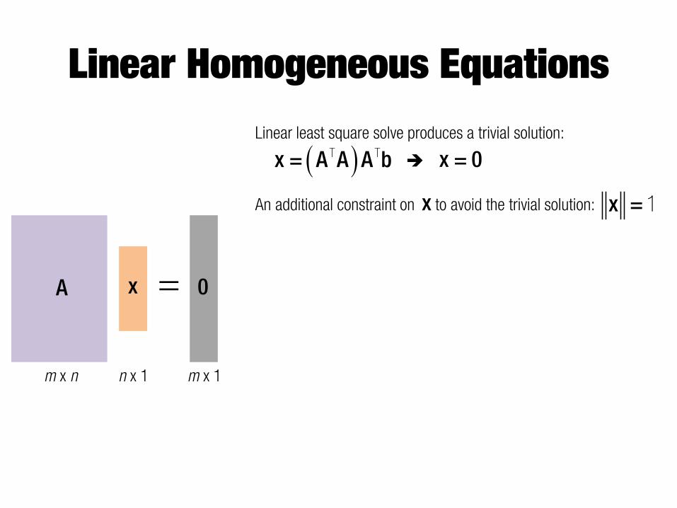
Linear Homogeneous Equations

= A x 0

m x n n x 1 m x 1

Linear least square solve produces a trivial solution:

x = 0� �x = A A A bT TÎ

An additional constraint on to avoid the trivial solution: x x = 1


= A x 0

m x n n x 1 m x 1


x = 0� �x = A A A bT TÎ


rank(A) = <r n -1 : infinite number of solutions

x = V + + Vr r n n"Ȝ Ȝ+1 +1 ¦

n

ii = r

Ȝ2+1

1where

1)


= A x 0

m x n n x 1 m x 1


x = 0� �x = A A A bT TÎ



x = V + + Vr r n n"Ȝ Ȝ+1 +1

rank(A) = n -1 : one exact solution

x = Vn

¦n

ii = r

Ȝ2+1

1where

1)

2)


= A x 0

m x n n x 1 m x 1


x = 0� �x = A A A bT TÎ



x = V + + Vr r n n"Ȝ Ȝ+1 +1

rank(A) = n -1 : one exact solution

x = Vn

¦n

ii = r

Ȝ2+1

1where

�n m : no exact solution in general (needs least squares)

xmin Ax 2

Î subject to x = 1 x = Vn

1)

2)

3)

• Distance between point (xn, yn) and line ax+by=d

• Find (a, b, d) to minimize the sum of squared perpendicular distances

ax+by=d

¦ ��

n

i ii dybxaE1

2)((xi, yi)

0N)UU( T data model parameters


2

664

x1 y1 �1x2 y2 �1· · · · · · �1xm ym �1

3

775 = 0

2

4abd

3

5

4

19

Demonstration

Let C(x) = 1� kxk2 be the constraint

Let E(x) = kAxk2 be the cost function

We must have:

(L(x

= 0 and(L(

= 0

The lagrangian is L(x) = E(x) + C(x), with a Lagrange multiplier

20

Demonstration

(L(x

= 2ATAx� 2x and(L(

= 1� kxk2 = C(x)

We get:

From which:

ATAx = x and C(x) = 0

p is an eigenvalue of ATA and x an (normalized) eigenvector

p is a squared singular value of A and x a singular vector

Asvd�� UVT

Let an SVD (Singular Value Decomposition) of matrix A be:

We have x = vi with i ; {1, . . . , n}

21

DemonstrationPlug x = vi back in the cost function E(x) = kAxk2:

E(vi) = kAvik2 = kUVTvik2

Since V is an orthonormal matrix, VTvi = ei (ei is a zero vectorwith one at the i-th entry):

E(vi) = kUeik2 = kU�ieik2

Let U = (u1 · · · un), we get:

E(vi) = k�iuik2 = �2i kuik2

Given that U is orthonormal:

E(vi) = �2i

We therefore choose for x the singular vector associated to thesmallest singular value, which concludes the proof. 22

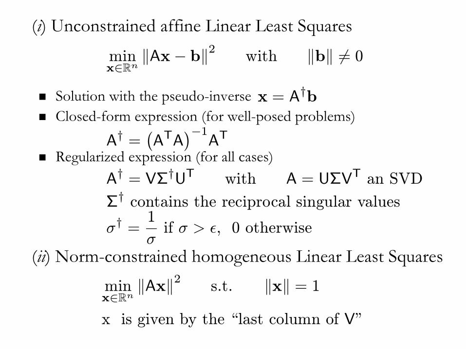
Summary and Closure� (i) Unconstrained affine Linear Least Squares

� Solution with the pseudo-inverse� Closed-form expression (for well-posed problems)

� Regularized expression (for all cases)


minx;Rn

kAx � bk2 with kbk 6= 0

x = A†b

A† =¡ATA

¢�1AT

A† = V†UT with A = UVT an SVD

† contains the reciprocal singular values

minx;Rn

kAxk2 s.t. kxk = 1

�† =1

�if � > ², 0 otherwise

x is given by the “last column of V”

23

A Quick Exercise

We define

mX

j=1

(yj � p(xj))2 � min

The goal of the exercise is to show how to fit apolynomial p of degree z to these points so that

p(x) =

zX

i=0

aixi

Let {(xj , yj)} be a set of 2D points, with j = 1, . . . , m

24

Questions

� Show that there exists a Linear Least Squares solution to this problem� Give the design matrix� Explain how to obtain the unknown coefficients

� What is the cost function minimized by the Linear Least Squares solution? how do you interpret it?

Homography Linear Estimation

x = Hx2 1

ª º« » « »« »¬ ¼

xuv1

1 1

1

ª º« » « »« »¬ ¼

Hh h hh h hh h h

11 12 13

21 22 23

31 32 33

ª º« » « »« »¬ ¼

xuv2

2 2

1

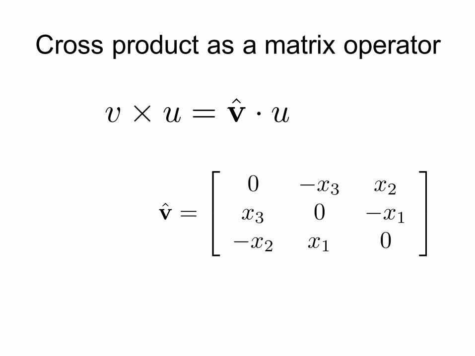
Cross product as a matrix operator

v ⇥ u = v̂ · u

v̂ =

2

40 �x3 x2

x3 0 �x1

�x2 x1 0

3

5

Homography Linear Estimation

x = Hx2 1

ª º« » « »« »¬ ¼

xuv1

1 1

1

> @u x Hx 02 1

u

�ª º ª º ª º« » « » « » � « » « » « »« » « » « »�¬ ¼ ¬ ¼ ¬ ¼

h h x h xh x h x h x 0h h x h x

u vv u

u v

2 1 2 3 1 2 1

2 2 1 1 1 2 3 1

3 2 2 1 2 1 11

u

u

u

ª º ª º�« » « »� « » « »« » « »�¬ ¼ ¬ ¼

0 x x hx 0 x h 0x x 0 h

vu

v u

T T T1 3 1 2 1 1T T T1 1 3 2 1 2

T T T2 1 2 1 1 3 3

3 x 9

rank( ) = 2 > @ux2because is a rank 2 matrix.

Therefore, 4 point correspondences are required to estimate a homography.

Fundamental Matrix Estimation

x FxT2 1 0

ª º« » « »« »¬ ¼

xuv1

1 1

1

ª º« » « »« »¬ ¼

xuv2

2 2

1

Fundamental Matrix Estimation x FxT

2 1 0

� � � � � � � � u u f u v f u f v u f v v f v f u f v f f2 1 11 2 1 12 2 13 2 1 21 2 1 22 2 23 1 31 1 32 33 0

ª º ª º ª º« » « » « » « » « » « »« » « » « »¬ ¼ ¬ ¼ ¬ ¼

u f f f uv f f f v

f f f

T

2 11 12 13 1

2 21 22 23 1

31 32 33

0

1 1

ª º« »« »« »« »

ª º « »« » « » « » « »« » « »¬ ¼

« »« »« »« »¬ ¼

0

fff

u u u v u v u v v v u v ffffff

# # # # # # # # #

11

12

13

2 1 2 1 2 2 1 2 1 2 1 1 21

22

23

31

32

33

1

9

Therefore, 8 point correspondences are required to estimate a fundamental matrix.

Problem: squared error heavily penalizes outliers

Least squares: Robustness to noise

outlier!

SilvioSavarese

Least Square ++ Camera 3D Registration 3D triangulation...

Documents

Transcript of Least Square ++ Camera 3D Registration 3D triangulation...